Efficient Mixed-Norm Regularization: Algorithms and Safe Screening ...

Efficient Mixed-Norm Regularization: Algorithms and Safe Screening Methods Jie Wang1 , Jun Liu1 , and Jieping Ye1

arXiv:1307.4156v1 [cs.LG] 16 Jul 2013

1

Computer Science and Engineering, Arizona State University, USA July 17, 2013

Abstract Sparse learning has recently received increasing attention in many areas including machine learning, statistics, and applied mathematics. The mixed-norm regularization based on the ℓ1 /ℓq norm with q > 1 is attractive in many applications of regression and classification in that it facilitates group sparsity in the model. The resulting optimization problem is, however, challenging to solve due to the inherent structure of the ℓ1 /ℓq -regularization. Existing work deals with special cases including q = 2, ∞, and they can not be easily extended to the general case. In this paper, we propose an efficient algorithm based on the accelerated gradient method for solving the ℓ1 /ℓq -regularized problem, which is applicable for all values of q larger than 1, thus significantly extending existing work. One key building block of the proposed algorithm is the ℓ1 /ℓq -regularized Euclidean projection (EP1q ). Our theoretical analysis reveals the key properties of EP1q and illustrates why EP1q for the general q is significantly more challenging to solve than the special cases. Based on our theoretical analysis, we develop an efficient algorithm for EP1q by solving two zero finding problems. To further improve the efficiency of solving large dimensional ℓ1 /ℓq regularized problems, we propose an efficient and effective “screening” method which is able to quickly identify the inactive groups, i.e., groups that have 0 components in the solution. This may lead to substantial reduction in the number of groups to be entered to the optimization. An appealing feature of our screening method is that the data set needs to be scanned only once to run the screening. Compared to that of solving the ℓ1 /ℓq -regularized problems, the computational cost of our screening test is negligible. The key of the proposed screening method is an accurate sensitivity analysis of the dual optimal solution when the regularization parameter varies. Experimental results demonstrate the efficiency of the proposed algorithm.

1

Introduction

Regularization has played a central role in many machine learning algorithms. The ℓ1 -regularization has recently received increasing attention, due to its sparsity-inducing property, convenient convexity, strong theoretical guarantees, and great empirical success in various applications. A well-known application of the ℓ1 -regularization is the Lasso [37]. Recent studies in areas such as machine learning, statistics, and applied mathematics have witnessed growing interests in extending the ℓ1 -regularization to the ℓ1 /ℓq regularization [2, 8, 17, 26, 32, 35, 41, 45, 46]. This leads to the following ℓ1 /ℓq -regularized minimization problem: minp f (W) ≡ l(W) + λ̟(W), (1) W∈R

where W ∈ Rp denotes the model parameters, l(·) is a convex loss dependent on the training samples and their corresponding responses, W = [w1T , w2T , . . . , wsT ]T is divided into s non-overlapping groups, wi ∈ Rpi , i = 1, 2. . . . , s, λ > 0 is the regularization parameter, and ̟(W) =

s X i=1

1

kwi kq

(2)

is the ℓ1 /ℓq norm with k · kq denoting the vector ℓq norm (q ≥ 1). One of the commonly used loss function is the least square loss, i.e., l(W) takes the form as

2

s

X 1 1

2 l(W) = kY − BWk2 = Y − Bi w i , (3)

2 2 i=1

2

m×p

where B = [B1 , B2 , . . . , Bs ] ∈ R is the data matrix with m samples and p features, Bi ∈ Rm×pi , i = 1, 2, . . . , s, is corresponding to the ith group, and Y ∈ Rm denotes the response vector. The ℓ1 /ℓq regularization belongs to the composite absolute penalties (CAP) [46] family. When q = 1, the problem (1) reduces to the ℓ1 -regularized problem. When q > 1, the ℓ1 /ℓq -regularization facilitates group sparsity in the resulting model, which is desirable in many applications of regression and classification. The practical challenge in the use of the ℓ1 /ℓq -regularization lies in the development of efficient algorithms for solving (1), due to the non-smoothness of the ℓ1 /ℓq -regularization. According to the black-box Complexity Theory [28, 29], the optimal first-order black-box method [28, 29] for solving the class of nonsmooth convex problems converges as O( √1k ) (k denotes the number of iterations), which is slow. Existing algorithms focus on solving the problem (1) or its equivalent constrained version for q = 2, ∞, and they can not be easily extended to the general case. In order to systematically study the practical performance of the ℓ1 /ℓq regularization family, it is of great importance to develop efficient algorithms for solving (1) for any q larger than 1.

1.1

First-Order Methods Applicable for (1)

When treating f (·) as the general non-smooth convex function, we can apply the subgradient descent (SD) [6, 28, 29]: Xi+1 = Xi − γi Gi , (4)

where Gi ∈ ∂f (Xi ) is a subgradient of f (·) at Xi , and γi a step size. There are several different types of step size rules, and more details can√be found in [6, 28]. Subgradient descent is proven to converge, and it can yield a convergence rate of O(1/ k) for k iterations. However, SD has the following two disadvantages: 1) SD converges slowly; and 2) the iterates of SD are very rarely at the points of non-differentiability [8], thus it might not achieve the desirable sparse solution (which is usually at the point of non-differentiability) within a limited number of iterations. Coordinate Descent (CD) [39] and its recent extension—Coordinate Gradient Descent (CGD) can be applied for optimizing the non-differentiable composite function [40]. Coordinate descent has been applied for the ℓ1 -norm regularized least squares [11], ℓ1 /ℓ∞ -norm regularized least squares [19], and the sparse group Lasso [10]. Coordinate gradient descent has been applied for the group Lasso logistic regression [24]. Convergence results for CD and CGD have been established, when the non-differentiable part is separable [39, 40]. However, there is no global convergence rate for CD and CGD (Note, CGD is reported to have a local linear convergence rate under certain conditions [40, Theorem 4]). In addition, it is not clear whether CD and CGD are applicable to the problem Eq. (1) with an arbitrary q ≥ 1. Fixed Point Continuation [15, 34] was recently proposed for solving the ℓ1 -norm regularized optimization (i.e., ̟(W) = kWk1 ). It is based on the following fixed point iteration: ̟ Xi+1 = Pλτ (Xi − τ l′ (Xi )),

(5)

̟ where Pλτ (W) = sgn(W) ⊙ max(W − λτ, 0) is an operator and τ > 0 is the step size. The fixed point ̟ iteration Eq. (5) can be applied to solve Eq. (1) for any convex penalty ̟(W), with the operator Pλτ (·) being defined as: 1 ̟ Pλτ (W) = arg min kX − Wk22 + λτ ϕ(X). (6) X 2 ̟ The operator Pλτ (·) is called the proximal operator [16, 25, 44], and is guaranteed to be non-expansive. With a properly chosen τ , the fixed point iteration Eq. (5) can converge to the fixed point X∗ satisfying ̟ X∗ = Pλτ (X∗ − τ l′ (X∗ )).

2

(7)

It follows from Eq. (6) and Eq. (7) that, 0 ∈ X∗ − (X∗ − τ l′ (X∗ )) + λτ ∂̟(X∗ ),

(8)

which together with τ > 0 indicates that X∗ is the optimal solution to Eq. (1). In [3, 30], the gradient descent method is extended to optimize the composite function in the form of Eq. (1), and the iteration step is similar to Eq. (5). The extended gradient descent method for nonsmooth objective functions is proven to yield the convergence rate of O(1/k) for k iterations. However, as pointed out in [3, 30], the scheme in Eq. (5) can be further accelerated for solving Eq. (1). Finally, there are various online learning algorithms that have been developed for dealing with large scale data, e.g., the truncated gradient method [18], the forward-looking subgradient [8], and the regularized dual averaging [43] (which is based on the dual averaging method proposed in [31]). When applying the ̟ aforementioned online learning methods for solving Eq. (1), a key building block is the operator Pλτ (·).

1.2

Screening Methods for (1)

Although many algorithms have been proposed to solve the mixed norm regularized problems, it remains challenging to solve especially for large-scale problems. To address this issue, “screening” has been shown to be a promising approach. The key idea of screening is to first identify the “inactive” features/groups, which have 0 coefficients in the solution. Then the inactive features/groups can be discarded from the optimization, leading to a reduced feature matrix and substantial savings in computational cost and memory size. In [12], El Ghaoui et al. proposed novel screening methods, called “SAFE”, to improve the efficiency for solving a class of ℓ1 regularized problems, including Lasso, ℓ1 regularized logistic regression and ℓ1 regularized support vector machines. Inspired by SAFE, Tibshirani et al. [38] proposed “strong rules” for a large class of ℓ1 regularized problems, including Lasso, ℓ1 regularized logistic regression, ℓ1 /ℓq regularized problems and more general convex problems. Although in most of the cases strong rules are more effective in discarding features than SAFE, it is worthwhile to note that strong rules may mistakenly discard features that have non-zero coefficients in the solution. To overcome this limitation, in [42] the authors proposed the “DPP” rules for the group Lasso problem [45], that is, the ℓ1 /ℓq -regularization problem in which q = 2. The DPP rules are safe in the sense that the features/groups discarded from the optimization are guaranteed to have 0 coefficients in the solution. The core of strong rules for the ℓ1 /ℓq problems is the assumption that the function ∇l(X∗ (λ)), that is, the gradient of the loss function l(·) at the optimal solution X∗ (λ) of problem Eq. (1), is a Lipschitz function of λ. However, this assumption does not always hold in practice [38]. Therefore, groups which have non-zero coefficients can be discarded mistakenly by strong rules. The key idea of DPP rules is to bound the dual optimal solution of problem Eq. (1) within a region R and compute maxθ∈R kBiT θkq¯, i = 1, 2, . . . , s, where 1/q + 1/¯ q = 1 (recall that Bi is the data matrix corresponding to wi ). The smaller the region R is, the more inactive groups can be detected. In this paper, we give a more accurate estimation of the region R and extend the idea to the general case with q ≥ 1.

1.3

Main Contributions

The main contributions of this paper include the following two parts. 1. We develop an efficient algorithm for solving the ℓ1 /ℓq -regularized problem (1), for any q ≥ 1. More specifically, we develop the GLEP1q algorithm1 , which makes use of the accelerated gradient method [3, 30] for minimizing the composite objective functions. GLEP1q has the following two favorable properties: (1) It is applicable to any smooth convex loss l(·) (e.g., the least squares loss and the logistic loss) and any q ≥ 1. Existing algorithms are mainly focused on ℓ1 /ℓ2 -regularization and/or ℓ1 /ℓ∞ -regularization. To the best of our knowledge, this is the first work that provides an efficient algorithm for solving (1) with any q ≥ 1; and (2) It achieves a global convergence rate of O( k12 ) (k 1 GLEP

1q

stands for Group Sparsity Learning via the ℓ1 /ℓq -regularized Euclidean Projection.

3

denotes the number of iterations) for the smooth convex loss l(·). In comparison, although the methods proposed in [1, 7, 19, 32] converge, there is no known convergence rate; and the method proposed in [24] has a local linear convergence rate under certain conditions [40, Theorem 4]. In addition, these methods are not applicable for an arbitrary q ≥ 1.

The main technical contribution of the proposed GLEP1q is the development of an efficient algorithm for computing the ℓ1 /ℓq -regularized Euclidean projection (EP1q ), which is a key building block in the GLEP1q algorithm. More specifically, we analyze the key theoretical properties of the solution of EP1q , based on which we develop an efficient algorithm for EP1q by solving two zero finding problems. In addition, our theoretical analysis reveals why EP1q for the general q is significantly more challenging than the special cases such as q = 2. We have conducted experimental studies to demonstrate the efficiency of the proposed algorithm. 2. We develop novel screening methods for large-scale mixed-norm (Smin) regularized problems. The proposed screening method is able to quickly identify the inactive groups, i.e., groups that have 0 components in the solution. Consequently, the inactive groups can be removed from the optimization problem and the scale of the resulting problem can be significantly reduced. Several appealing features of our screening method includes: (1) It is “safe” in the sense that the groups removed from the optimization are guaranteed to have 0 components in the solution. (2) The data set needs to be scanned only once to run the screening. (3) The computational cost of the proposed screening rule is negligible compared to that of solving the ℓ1 /ℓq -regularized problems. (4) Our screening method is independent of solvers for the ℓ1 /ℓq -regularized problems and thus it can be integrated with any existing solver to improve the efficiency. Due to the difficulty of the ℓ1 /ℓq -regularized problems, existing screening methods are limited to [38, 42]. In comparison, the method proposed in [38] is “inexact” in the sense that it may mistakenly remove groups from the optimization which have nonzero coefficients in the solution; and the method proposed in [42] is designed for the case q = 2. The key of the proposed screening method is an accurate estimation of the region R which includes the dual optimal solution of problem Eq. (1) via the “variational inequalities” [13]. After the upper bound maxθ∈R kBiT θkq¯ is computed, we make use of the KKT condition to determine if the ith group has 0 coefficients in the solution and can be removed from the optimization. Experimental results show that the efficiency of the proposed GLEP1q can be improved by “three orders of magnitude” with the screening method, especially for the large dimensional data sets.

1.4

Related Work

We briefly review recent studies on ℓ1 /ℓq -regularization and the corresponding screening methods, most of which focus on ℓ1 /ℓ2 -regularization and/or ℓ1 /ℓ∞ -regularization. ℓ1 /ℓ2 -Regularization: The group Lasso was proposed in [45] to select the groups of variables for prediction in the least squares regression. In [24], the idea of group lasso was extended for classification by the logistic regression model, and an algorithm via the coordinate gradient descent [40] was developed. In [32], the authors considered joint covariate selection for grouped classification by the logistic loss, and developed a blockwise boosting Lasso algorithm with the boosted Lasso [47]. In [1], the authors proposed to learn the sparse representations shared across multiple tasks, and designed an alternating algorithm. The Spectral projected-gradient (Spg) algorithm was proposed for solving the ℓ1 /ℓ2 -ball constrained smooth optimization problem [4], equipped with an efficient Euclidean projection that has expected linear runtime. The ℓ1 /ℓ2 regularized multi-task learning was proposed in [21], and the equivalent smooth reformulations were solved by the Nesterov’s method [29]. ℓ1 /ℓ∞ -Regularization: A blockwise coordinate descent algorithm [39] was developed for the mutli-task Lasso [19]. It was applied to the neural semantic basis discovery problem. In [33], the authors considered the multi-task learning via the ℓ1 /ℓ∞ -regularization, and proposed to solve the equivalent ℓ1 /ℓ∞ -ball constrained problem by the projected gradient descent. In [27], the authors considered the multivariate regression via the ℓ1 /ℓ∞ -regularization, showed that the high-dimensional scaling of ℓ1 /ℓ∞ -regularization is qualitatively 4

similar to that of ordinary ℓ1 -regularization, and revealed that, when the overlap parameter is large enough (> 2/3), ℓ1 /ℓ∞ -regularization yields the improved statistical efficiency over ℓ1 -regularization. ℓ1 /ℓq -Regularization: In [7], the authors studied the problem of boosting with structural sparsity, and developed several boosting algorithms for regularization penalties including ℓ1 , ℓ∞ , ℓ1 /ℓ2 , and ℓ1 /ℓ∞ . In [46], the composite absolute penalties (CAP) family was introduced, and an algorithm called iCAP was developed. iCAP employed the least squares loss and the ℓ1 /ℓ∞ regularization, and was implemented by the boosted Lasso [47]. The multivariate regression with the ℓ1 /ℓq -regularization was studied in [20]. In [26], a unified framework was provided for establishing consistency and convergence rates for the regularized M -estimators, and the results for ℓ1 /ℓq regularization was established. ℓ1 /ℓq -Screening: To the best of our knowledge, existing screening methods for ℓ1 /ℓq -Regularization are limited to the methods proposed in [38, 42]. The methods proposed in [38], i.e., the strong rules, assume that the gradient of the loss function at the optimal solution of problem Eq. (1) is a Lipschitz function of λ. However, there are counterexamples showing that the assumption can be violated in practice. As a result, groups which have non-zero coefficients in the solution can be mistakenly discarded from the optimization by strong rules. In [42], the authors considered the group lasso problem [45], that is, the ℓ1 /ℓ2 -regularized problems and proposed the DPP rules. The key idea of DPP rules is to estimate a region R which includes the dual optimal solution θ∗ (λ) of problem Eq. (1) by noting that θ∗ (λ) is nonexpansive with respect to λ.

1.5

Notation

Throughout this paper, scalars are denoted by italic letters, and vectors by bold face letters. Let X, Y, . . . denote the p-dimensional parameters, xi , yi , . . . the pi -dimensional parameters of the i-th group, and xi the q i-th component of x. We denote q¯ = q−1 , and thus q and q¯ satisfy the following relationship: 1q¯ + q1 = 1. We use the following componentwise operators: ⊙, .q , | · | and sgn(·). Specifically, z = x ⊙ y denotes zi = xi yi ; y = xq denotes yi = xqi ; y = |x| denotes yi = |xi |; and y = sgn(x) denotes yi = sgn(xi ), where sgn(·) Pis the signum function: sgn(t) = 1 if t > 0; sgn(t) = 0 if t = 0; and sgn(t) = −1 if t < 0. We use hx, yi = i xi yi to denote the inner product of x and y.

2

The Proposed GLEP1q Algorithm

In this paper, we consider solving Eq. (1) in the batch learning setting, and propose to apply the accelerated gradient method [3, 30] due to its fast convergence rate. We term our proposed algorithm as “GLEP1q ”, which stands for Group Sparsity Learning via the ℓ1 /ℓq -regularized Euclidean Projection. Note that, one can develop the online learning algorithm for Eq. (1) using the aforementioned online learning algorithms, where the ℓ1 /ℓq -regularized Euclidean projection is also a key building block. We first construct the following model for approximating the composite function M(·) at the point X: ML,X (Y) = [loss(X) + hloss′ (X), Y − Xi] + λ̟(Y) +

L kY − Xk22 , 2

(9)

where L > 0. In the model ML,X (Y), we apply the first-order Taylor expansion at the point X (including all terms in the square bracket) for the smooth loss function l(·), and directly put the non-smooth penalty ̟(·) into the model. The regularization term L2 kY − Xk22 prevents Y from walking far away from X, thus the model can be a good approximation to f (Y) in the neighborhood of X. The accelerated gradient method is based on two sequences {Xi } and {Si } in which {Xi } is the sequence of approximate solutions, and {Si } is the sequence of search points. The search point Si is the affine combination of Xi−1 and Xi as Si = Xi + βi (Xi − Xi−1 ), (10) where βi is a properly chosen coefficient. The approximate solution Xi+1 is computed as the minimizer of MLi ,Si (Y): (11) Xi+1 = arg min MLi ,Si (Y), Y

5

where Li is determined by line search, e.g., the Armijo-Goldstein rule so that Li should be appropriate for Si . Algorithm 1 GLEP1q : Group Sparsity Learning via the ℓ1 /ℓq -regularized Euclidean Projection Require: λ1 ≥ 0, λ2 ≥ 0, L0 > 0, X0 , k Ensure: Xk+1 1: Initialize X1 = X0 , α−1 = 0, α0 = 1, and L = L0 . 2: for i = 1 to k do i−2 −1 , Si = Xi + βi (Xi − Xi−1 ) 3: Set βi = αα i−1 4: Find the smallest L = Li−1 , 2Li−1 , . . . such that f (Xi+1 ) ≤ ML,Si (Xi+1 ), 5: 6:

where Xi+1 = arg minY M√ L,Si (Y)

Set Li = L and αi+1 = end for

1+

1+4α2i 2

The algorithm for solving Eq. (1) is presented in Algorithm 1. GLEP1q inherits the optimal convergence rate of O(1/k 2 ) from the accelerated gradient method. In Algorithm 1, a key subroutine is Eq. (11), which can be computed as Xi+1 = π1q (Si − l′ (Si )/Li , λ/Li ), where π1q (·) is the ℓ1 /ℓq -regularized Euclidean projection (EP1q ) problem: s X 1 kxi kq . (12) π1q (V, λ) = arg minp kX − Vk22 + λ X∈R 2 i=1

The efficient computation of Eq. (12) for any q > 1 is the main technical contribution of this paper. Note that the s groups in Eq. (12) are independent. Thus the optimization in (12) decouples into a set of s independent ℓq -regularized Euclidean projection problems:   1 πq (v) = arg minn g(x) = kx − vk22 + λkxkq , (13) x∈R 2 where n = pi for the i-th group. Next, we study the key properties of (13).

2.1

Properties of the Optimal Solution to (13)

The function g(·) is strictly convex, and thus it has a unique minimizer, as summarized below: Lemma 1. The problem (13) has a unique minimizer. Next, we show that the optimal solution to (13) is given by zero under a certain condition, as summarized in the following theorem: Theorem 2. πq (v) = 0 if and only if λ ≥ kvkq¯.

Proof. Let us first compute the directional derivative of g(x) at the point 0: Dg(0)[u] = lim α↓0

1 [g(αu) − g(0)] = −hv, ui + λkukq , α

where u is a given direction. According to the H¨ older’s inequality, we have |hu, vi| ≤ kukq kvkq¯, ∀u. Therefore, we have Dg(0)[u] ≥ 0, ∀u,

(14)

if and only if λ ≥ kvkq¯. The result follows, since (14) is the necessary and sufficient condition for 0 to be the optimal solution of (13). 6

q=1.5, λ=2

q=3, λ=2

3

1.5

1

1

x1

x

1

2

0

−1

0.5

0

10

20 30 iteration

40

−0.5

50

10

20 30 iteration

40

50

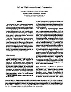
Figure 1: Illustration of the failure of the fixed point iteration x = v − λkxk1−q x(q−1) for solving (13). We set q v = [1, 3]T and the starting point x = [1, 3]T . The vertical axis denotes the values of x1 during the iterations.

Next, we focus on solving (13) for 0 < λ < kvkq¯. We first consider solving (13) in the case of 1 < q < ∞, which is the main technical contribution of this paper. We begin with a lemma that summarizes the key properties of the optimal solution to the problem (13): Lemma 3. Let 1 < q < ∞ and 0 < λ < kvkq¯. Then, x∗ is the optimal solution to the problem (13) if and if only it satisfies: (15) x∗ + λkx∗ k1−q x∗ (q−1) = v, q where y ≡ x(q−1) is defined component-wisely as: yi = sgn(xi )|xi |q−1 . Moreover, we have πq (v) = sgn(v) ⊙ πq (|v|),

(16)

sgn(x∗ ) = sgn(v),

(17)

0 < |x∗i | < |vi |, ∀i ∈ {i|vi 6= 0}.

(18)

Proof. Since λ < kvkq¯, it follows from Theorem 2 that the optimal solution x∗ 6= 0. kxkq is differentiable when x 6= 0, so is g(x). Therefore, the sufficient and necessary condition for x∗ to be the solution of (13) is g ′ (x∗ ) = 0, i.e., (15). Denote c∗ ≡ λkx∗ k1−q > 0. It follows from (15) that (16) holds, and q
sgn(x∗i ) |x∗i | + c∗ |x∗i |q−1 = vi ,

(19)

from which we can verify (17) and (18).

It follows from Lemma 3 that i) if vi = 0 then x∗i = 0; and ii) πq (v) can be easily obtained from πq (|v|). Thus, we can restrict our following discussion to v > 0, i.e., vi > 0, ∀i. It is clear that, the analysis can be easily extended to the general v. The optimality condition in (15) indicates that x∗ might be solved via the fixed point iteration x = η(x) ≡ v − λkxk1−q x(q−1) , q which is, however, not guaranteed to converge (see Figure 1 for examples), as η(·) is not necessarily a contraction mapping [17, Proposition 3]. In addition, x∗ cannot be trivially solved by firstly guessing c = kxk1−q and then finding the root of x + λcx(q−1) = v, as when c increases, the values of x obtained from q x + λcx(q−1) = v decrease, so that c = kxk1−q increases as well (note, 1 − q < 0). q

2.2

Computing the Optimal Solution x∗ by Zero Finding

In the following, we show that x∗ can be obtained by solving two zero finding problems. Below, we construct our first auxiliary function hvc (·) and reveal its properties:

7

Definition 4 (Auxiliary Function hvc (·) ). Let c > 0, 1 < q < ∞, and v > 0. We define the auxiliary function hvc (·) as follows: hvc (x) = x + cxq−1 − v, 0 ≤ x ≤ v. (20) Lemma 5. Let c > 0, 1 < q < ∞, and v > 0. Then, hvc (·) has a unique root in the interval (0, v). Proof. It is clear that hvc (·) is continuous and strictly increasing in the interval [0, v], hvc (0) = −v < 0, and hvc (v) = cv q−1 > 0. According to the Intermediate Value Theorem, hvc (·) has a unique root lying in the interval (0, v). This concludes the proof. Corollary 6. Let x, v ∈ Rn , c > 0, 1 < p < ∞, and v > 0. Then, the function ϕvc (x) = x + cx(q−1) − v, 0 < x < v

(21)

has a unique root. Let x∗ be the optimal solution satisfying (15). Denote c∗ = λkx∗ k1−q . It follows from Lemma 3 and q Corollary 6 that x∗ is the unique root of ϕvc∗ (·) defined in (21), provided that the optimal c∗ is known. Our methodology for computing x∗ is to first compute the optimal c∗ and then compute x∗ by computing the root of ϕvc∗ (·). Next, we show how to compute the optimal c∗ by solving a single variable zero finding problem. We need our second auxiliary function ω(·) defined as follows: Definition 7 (Auxiliary Function ω(·)). Let 1 < q < ∞ and v > 0. We define the auxiliary function ω(·) as follows: c = ω(x) = (v − x)/xq−1 , 0 < x ≤ v. (22) Lemma 8. In the interval (0, v], c = ω(x) is i) continuously differentiable, ii) strictly decreasing, and iii) invertible. Moreover, in the domain [0, ∞), the inverse function x = ω −1 (c) is continuously differentiable and strictly decreasing. Proof. It is easy to verify that, in the interval (0, v], c = ω(x) is continuously differentiable with a non-positive gradient, i.e., ω ′ (x) < 0. Therefore, the results follow from the Inverse Function Theorem. It follows from Lemma 8 that given the optimal c∗ and v, the optimal x∗ can be computed via the inverse function ω −1 (·), i.e., we can represent x∗ as a function of c∗ . Since λkx∗ k1−q − c∗ = 0 by the definition of q ∗ ∗ c , the optimal c is a root of our third auxiliary function φ(·) defined as follows: Definition 9 (Auxiliary Function φ(·)). Let 1 < q < ∞, 0 < λ < kvkq¯, and v > 0. We define the auxiliary function φ(·) as follows: φ(c) = λψ(c) − c, c ≥ 0, (23) where ψ(c) =

n X

(ωi−1 (c))q

i=1

and ωi−1 (c) is the inverse function of

! 1−q q

,

ωi (x) = (vi − x)/xq−1 , 0 < x ≤ vi .

(24)

(25)

Recall that we assume 0 < λ < kvkq¯ (otherwise the optimal solution is given by zero from Theorem 2). The following lemma summarizes the key properties of the auxiliary function φ(·): Lemma 10. Let 1 < q < ∞, 0 < λ < kvkq¯, v > 0, and ǫ = (kvkq¯ − λ)/kvkq¯.

8

(26)

Then, φ(·) is continuously differentiable in the interval [0, ∞). Moreover, we have φ(0) = λkvk1−q > 0, φ(c) ≤ 0, q

where c = max ci ,

(27)

ci = ωi (vi ǫ), i = 1, 2, . . . , n.

(28)

i

Proof. From Lemma 8, the function ωi−1 (c) is continuously differentiable in [0, ∞). It is easy to verify that ωi−1 (c) > 0, ∀c ∈ [0, ∞). Thus, φ(·) in (23) is continuously differentiable in [0, ∞). It is clear that φ(0) = λkvk1−q > 0. Next, we show φ(c) ≤ 0. Since 0 < λ < kvkq¯, we have q 0 < ǫ < 1.

(29)

It follows from (25), (27), (28) and (29) that 0 < ci ≤ c, ∀i. Let x = [x1 , x2 , . . . , xn ]T be the root of ϕvc (·) (see Corollary 6). Then, xi = ωi−1 (c). Since ωi−1 (·) is strictly decreasing (see Lemma 8), ci ≤ c, vi ǫ = ωi−1 (ci ), and xi = ωi−1 (c), we have xi ≤ vi ǫ. (30)

Combining (25), (30), and c = ωi (xi ), we have c ≥ vi (1 − ǫ)/xiq−1 , since ωi (·) is strictly decreasing. It follows 1   q−1 that xi ≥ vi (1−ǫ) . Thus, the following holds: c ψ(c) =

n X

(ωi−1 (c))q

i=1

! 1−q q

which leads to φ(c) = λψ(c) − c ≤ c where the last equality follows from (26).

n X

=

i=1



xqi

! 1−q q

≤

λ −1 kvkq¯(1 − ǫ)

c , kvkq¯(1 − ǫ)



= 0,

Corollary 11. Let 1 < q < ∞, 0 < λ < kvkq¯, v > 0, and c = mini ci , where ci ’s are defined in (28). We have 0 < c ≤ c and φ(c) ≥ 0. Following Lemma 10 and Corollary 11, we can find at least one root of φ(·) in the interval [c, c]. In the following theorem, we show that φ(·) has a unique root: Theorem 12. Let 1 < q < ∞, 0 < λ < kvkq¯, and v > 0. Then, in [c, c], φ(·) has a unique root, denoted by c∗ , and the root of ϕvc∗ (·) is the optimal solution to (13). Proof. From Lemma 10 and Corollary 11, we have φ(c) ≤ 0 and φ(c) ≥ 0. If either φ(c) = 0 or φ(c) = 0, c or c is a root of φ(·). Otherwise, we have φ(c)φ(c) < 0. As φ(·) is continuous in [0, ∞), we conclude that φ(·) has a root in (c, c) according to the Intermediate Value Theorem. Next, we show that φ(·) has a unique root in the interval [0, ∞). We prove this by contradiction. Assume that φ(·) has two roots: 0 < c1 < c2 . From Corollary 6, ϕvc1 (·) and ϕvc2 (·) have unique roots. Denote x1 = [x11 , x12 , . . . , x1n ]T and x2 = [x21 , x22 , . . . , x2n ]T as the roots of ϕvc1 (·) and ϕvc2 (·), respectively. We have 0 < x1i , x2i < vi , ∀i. It follows from (23-25) that x1 + λkx1 k1−q x1 q 2

x +

(q−1)

(q−1) λkx2 k1−q x2 q

− v = 0, − v = 0.

According to Lemma 3, x1 and x2 are the optimal solution of (13). From Lemma 1, we have x1 = x2 . However, since x1i = ωi−1 (c1 ), x2i = ωi−1 (c2 ), ωi−1 (·) is a strictly decreasing function in [0, ∞) by Lemma 8, and c1 < c2 , we have x1i > x2i , ∀i. This leads to a contradiction. Therefore, we conclude that φ(·) has a unique root in [c, c]. From the above arguments, it is clear that, the root of ϕvc∗ (·) is the optimal solution to (13). 9

Remark 13. When q = 2, we have c = c =

λ kvk2 −λ .

π2 (v) =

It is easy to verify that φ(c) = φ(c) = 0 and kvk2 − λ v. kvk2

(31)

Therefore, when q = 2, we obtain a closed-form solution.

2.3

Solving the Zero Finding Problem by Bisection

Let 1 < q < ∞, 0 < λ < kvkq¯, v > 0, v = maxi vi , v = mini vi , and δ > 0 be a small constant (e.g., δ = 10−8 in our experiments). When q > 2, we have c=

1−ǫ ǫq−1 v q−2

and

c=

1−ǫ . ǫq−1 v q−2

c=

1−ǫ ǫq−1 v q−2

and

c=

1−ǫ . ǫq−1 v q−2

When 1 < q < 2, we have

If either φ(c) = 0 or φ(c) = 0, c or c is the unique root of φ(·). Otherwise, we can find the unique root of φ(·) by bisection in the interval (c, c), which costs at most N = log2

(1 − ǫ)|v q−2 − v q−2 | ǫq−1 v q−2 v q−2 δ

iterations for achieving an accuracy of δ. Let [c1 , c2 ] be the current interval of uncertainty, and we have 2 computed ωi−1 (c1 ) and ωi−1 (c2 ) in the previous bisection iterations. Setting c = c1 +c 2 , we need to evaluate −1 −1 φ(c) by computing ωi (c), i = 1, 2, . . . , n. It is easy to verify that ωi (c) is the root of hvc i (·) in the interval (0, vi ). Since ωi−1 (·) is a strictly decreasing function (see Lemma 8), the following holds: ωi−1 (c2 ) < ωi−1 (c) < ωi−1 (c1 ), and thus ωi−1 (c) can be solved by bisection using at most log2

vi v ωi−1 (c2 ) − ωi−1 (c1 ) < log2 ≤ log2 δ δ δ

iterations for achieving an accuracy of δ. For given v, λ, and δ, N and v are constant, and thus it costs O(n) for finding the root of φ(·). Once c∗ , the root of φ(·) is found, it costs O(n) flops to compute x∗ as the unique root of ϕvc∗ (·). Therefore, the overall time complexity for solving (13) is O(n). We have shown how to solve (13) for 1 < q < ∞. For q = 1, the problem (13) is reduced to the one used in the standard Lasso, and it has the following closed-form solution [3]: π1 (v) = sgn(v) ⊙ max(|v| − λ, 0).

(32)

For q = ∞, the problem (13) can computed via Eq. (32), as summarized in the following theorem: Theorem 14. Let q = ∞, q¯ = 1, and 0 < λ < kvkq¯. Then we have π∞ (v) = sgn(v) ⊙ min(|v|, t∗ ), where t∗ is the unique root of h(t) =

n X i=1

max(|vi | − t, 0) − λ.

10

(33)

(34)

Proof. Making use of the property that kxk∞ = maxkyk1 ≤1 hy, xi, we can rewrite (13) in the case of q = ∞ as 1 (35) min max s(x, y) ≡ kx − vk22 + hy, xi. x y:kyk1 ≤λ 2 The function s(x, y) is continuously differentiable in both x and y, convex in x and concave in y, and the feasible domains are solids. According to the well-known von Neumann Lemma [28], the min-max problem (35) has a saddle point, and thus the minimization and maximization can be exchanged. Setting the derivative of s(x, y) with respect to x to zero, we have x = v − y. Thus we obtain the following problem: min

y:kyk1 ≤λ

(36)

1 ky − vk22 , 2

(37)

which is the problem of the Euclidean projection onto the ℓ1 ball [4, 7, 23]. It has been shown that the optimal solution y∗ to (37) for λ < kvk1 can be obtained by first computing t∗ as the unique root of (34) in linear time, and then computing y∗ as y∗ = sgn(v) ⊙ max(|v| − t∗ , 0).

(38)

It follows from (36) and (38) that (33) holds. We conclude this section by summarizing the results for solving the ℓq -regularized Euclidean projection in Algorithm 2. Algorithm 2 Epq : ℓq -regularized Euclidean projection Require: λ > 0, q ≥ 1, v ∈ Rn Ensure: x∗ = πq (v) = arg minx∈Rn 12 kx − vk22 + λkxkq q 1: Compute q¯ = q−1 2: if kvkq¯ ≤ λ then 3: Set x∗ = 0, return 4: end if 5: if q = 1 then 6: Set x∗ = sgn(v) ⊙ max(|v| − λ, 0) 7: else if q = 2 then 2 −λ 8: Set x∗ = kvk kvk2 v 9: else if q = ∞ then 10: Obtain t∗ , the unique root of h(t), via the improved bisection method [23] 11: Set x∗ = sgn(v) ⊙ min(|v|, t∗ ) 12: else 13: Compute c∗ , the unique root of φ(c), via bisection in the interval [c, c] 14: Obtain x∗ as the unique root of ϕvc∗ (·) 15: end if

3

The Proposed Screening Method (Smin) for the ℓ1/ℓq -regularized Problems

In this section, we assume the loss function ℓ(·) is the least square loss, i.e., we consider the following problem:

2

s s

X X 1

kwi kq . (39) Bi w i + λ minp f (W) = Y −

W∈R 2 i=1

11

2

i=1

The dual problem of (39) takes the form as: max θ

2

1 λ2

θ − Y , kY k22 −

2 2 λ 2

(40)

s.t. kBiT θkq¯ ≤ 1, i = 1, 2, . . . , s. Let X∗ (λ) and θ∗ (λ) be the optimal solutions of problems (39) and (40) respectively. The KKT conditions read as: s X Bi X∗i (λ) + λθ∗ (λ), (41) Y = i=1

BiT θ∗ (λ) ∈

(

X∗ i (λ) , kX∗ ¯ i (λ)kq

Ui , Ui ∈ Rpi , kUi kq¯ ≤ 1,

if X∗i (λ) 6= 0,

if X∗i (λ) = 0,

i = 1, 2, . . . , s.

(42)

In view of Eq. (42), we can see that kBiT θ∗ (λ)kq¯ < 1 ⇒ X∗i (λ) = 0.

(R)

In other words, if kBiT θ∗ (λ)kq¯ < 1, then the KKT conditions imply that the coefficients of Bi in the solution X∗ (λ), that is, X∗i (λ), are 0 and thus the ith group can be safely removed from the optimization of problem (39). However, since θ∗ (λ) is in general unknown, (R) is not very helpful to discard inactive groups. To this end, we will estimate a region R which contains θ∗ (λ). Therefore, if maxθ∈R kBiT θkq¯ < 1, we can also conclude that X∗i (λ) = 0 by (R). As a result, the rule in (R) can be relaxed as ϕ(θ∗ (λ), Bi ) := max kBiT θkq¯ < 1 ⇒ X∗i (λ) = 0. θ∈R

(R′ )

In this paper, (R′ ) serves as the cornerstone for constructing the proposed screening rules. From (R′ ), we can see that screening rules with smaller ϕ(θ∗ (λ), Bi ) are more effective in identifying inactive groups. To give a tight estimation of ϕ(θ∗ (λ), Bi ), we need to restrict the region R containing θ∗ (λ) as small as possible. In Section 3.1, we give an accurate estimation of the possible region of θ∗ (λ) via the variational inequality. We then derive the upper bound ϕ(θ∗ (λ), Bi ) in Section 3.2 and construct the proposed screening rules, that is, Smin, in Section 3.3 based on (R′ ).

3.1

Estimating the Possible Region for θ∗ (λ)

In this section, we briefly discuss the geometric properties of the optimal solution θ∗ (λ) of problem (40), and then give an accurate estimation of the possible region of θ∗ (λ) via the variational inequality. Consider problem

2 1 Y

min g(θ) := θ − , (43) θ 2 λ 2 s.t. kBiT θkq¯ ≤ 1, i = 1, 2, . . . , s.

It is easy to see that problems (40) and (43) have the same optimal solution. Let F = {θ : kBiT θkq¯ ≤ 1, i = 1, 2, . . . , s.} denote the feasible set of problem (43). We can see that the optimal solution θ∗ (λ) of problem (43) is the projection of Yλ onto the feasible set F . The following theorem shows that problem (39) and its dual (40) admit closed form solutions when λ is large enough. Theorem 15. Let X∗ (λ) and θ∗ (λ) be the optimal solutions of problem (39) and its dual (40). Then if λ ≥ λmax := maxi kBiT Y kq¯, we have X∗ (λ) = 0 and θ∗ (λ) =

12

Y . λ

(44)

Proof. We first consider the cases in which λ > λmax . When λ > λmax , we can see that kBiT Yλ kq¯ < 1 for all i = 1, 2, . . . , s, i.e., Yλ is itself an interior point of F . As a result, we have θ∗ (λ) = Yλ . Therefore, the rule in (R) implies that X∗i (λ) = 0, i = 1, 2, . . . , s, i.e., the optimal solution X∗ (λ) of problem (39) is 0. Next let us consider the case in which λ = λmax . Because F is convex and θ∗ (λ) is the projection of Yλ onto F , we can see that θ∗ (λ) is nonexpansive with respect to λ [5] and thus θ∗ (λ) is a continuous function of λ. Therefore, it is easy to see that θ∗ (λmax ) = lim θ∗ (λ) = λ↓λmax

Let h(λ) := BX∗ (λ) =

Ps

i=1

Y . λmax

Bi X∗i (λ). By Eq. (41), we have h(λ) = Y − λθ∗ (λ),

which implies that h(λ) is also continuous with respect to λ. Therefore, we have h(λmax ) = lim h(λ) = 0. λ↓λmax

Clearly, we can set X = 0 such that h(λmax ) = BX = 0 can be satisfied. Therefore, both of the KKT Y conditions in Eq. (41) and Eq. (42) are satisfied by X and θ∗ (λmax ) = λmax . Because problem (39) is a convex optimization problem, the satisfaction of the KKT conditions implies that X = 0 is an optimal ∗ solution of (39). Therefore, we can choose 0 for XP (λmax ). Moreover, we can see that X∗ (λmax ) must be s 1 2 ∗ zero because otherwise f (X (λmax )) = 2 kY k2 + λ i=1 kX∗i (λmax )kq¯ > 12 kY k22 = f (0). Therefore, we have X∗ (λmax ) = 0 which completes the proof. Suppose we are given two distinct parameters λ′ and λ′′ and the corresponding optimal solutions of (43) are θ∗ (λ′ ) and θ∗ (λ′′ ) respectively. Without loss of generality, let us assume λmax ≥ λ′ > λ′′ > 0. Then the variational inequalities [13] can be written as

Because ∇g(θ) = θ −

Y λ,

hθ∗ (λ′ ) − θ∗ (λ′′ ), ∇g(θ∗ (λ′′ ))i ≥ 0,

(45)

hθ∗ (λ′′ ) − θ∗ (λ′ ), ∇g(θ∗ (λ′ ))i ≥ 0.

(46)

the variational inequalities in Eq. (45) and Eq. (46) can be rewritten as:   Y θ∗ (λ′ ) − θ∗ (λ′′ ), θ∗ (λ′′ ) − ′′ ≥ 0, λ   Y ∗ ′′ ∗ ′ ∗ ′ θ (λ ) − θ (λ ), θ (λ ) − ′ ≥ 0. λ

(47) (48)

Y When λ′ = λmax , Theorem 15 tells that θ∗ (λ′ ) = θ∗ (λmax ) = λmax and thus the inequality in Eq. (48) is trivial. Let B∗ := argmaxi kBiT θ∗ (λmax )kq¯ and φ(θ) := kB∗T θkq¯ where θ ∈ Rm . Then the subdifferential of φ(·) can be found as: ∂φ(θ) := {B∗ d : kdkq ≤ 1, hd, B∗T θi = kB∗T θkq¯}.

To simplify notations, let θmax := θ∗ (λmax ). Consider ∂φ(θmax ). It is easy to see that B∗T θmax 6= 0 since kB∗T θmax kq¯ = 1. Let dmax = sgn(B∗T θmax ) ⊙ |B∗T θmax |q¯/q . (49)

It is easy to check that kdmax kq = 1 and hdmax , B∗T θmax i = kB∗T θmax kq¯ = 1, which implies that B∗ dmax ∈ ∂φ(θmax ). As a result, the hyperplane H := {θ ∈ Rm : hB∗ dmax , θi = kB∗T θkq¯ = 1} 13

(50)

is a supporting hyperplane [16] to the set C := {θ ∈ Rm : kB∗T θkq¯ ≤ 1}. As a result, H is also a supporting hyperplane to the set F . [Recall that F is the feasible set of problem (43) and C ⊆ F .] Therefore, when λ′ = λmax , we have hθ − θ∗ (λ′ ), −B∗ dmax i ≥ 0, ∀θ ∈ F .

(51)

Suppose θ∗ (λ′ ) is known, for notational convenience, let   1 Y ′′ ′ ∗ ′ a(λ , λ ) = − θ (λ ) , 2 λ′′ ( Y ∗ ′ if λ′ ∈ (0, λmax ) ′ − θ (λ ), ′ b(λ ) = λ B∗ dmax , if λ′ = λmax , v(λ′′ , λ′ ) = a(λ′′ , λ′ ) − and

(52)

(53)

ha(λ′′ , λ′ ), b(λ′ )i b(λ′ ), kb(λ′ )k22

o(λ′′ , λ′ ) = θ∗ (λ′ ) + v(λ′′ , λ′ ). ′′

(54)

(55)

′

′

The next lemma shows that the inner product between a(λ , λ ) and b(λ ) is nonnegative. Lemma 16. Suppose θ∗ (λ′ ) and θ∗ (λ′′ ) are the optimal solutions of problem (43) for two distinct parameters λmax ≥ λ′ > λ′′ > 0. Then ha(λ′′ , λ′ ), b(λ′ )i ≥ 0. (56) Proof. We first show that the statement holds when λ′ = λmax . Y By Theorem 15, we can see that θ∗ (λmax ) = λmax and thus a(λ′′ , λmax ) =

1 2



1 1 − λ′′ λmax



Y.

If Y = 0, the statement is trivial. Let us assume Y 6= 0. Then   1 1 1 hY, B∗ dmax i. ha(λ′′ , λmax ), b(λmax )i = − 2 λ′′ λmax

(57)

On the other hand, because the zero point is also a feasible point of problem (43), i.e., 0 ∈ F , we can see that Y , −B∗ dmax i ≥ 0. (58) h0 − θ∗ (λmax ), −B∗ dmax i = h− λmax In view of Eq. (57) and Eq. (58), we have ha(λ′′ , λmax ), b(λmax )i ≥ 0. Next, let us consider the case with 0 < λ′ < λmax . In fact, we can see that   Y ∗ ′ Y ∗ ′ − θ (λ ), − θ (λ ) h2a(λ′′ , λ′ ), b(λ′ )i = λ′′ λ′

2  ′  

Y

λ Y Y ∗ ′ ∗ ′

= −1 , − θ (λ ) + ′ − θ (λ ) λ′′ λ′ λ′ λ 2    ′ Y λ −1 θ∗ (λ′ ), ′ − θ∗ (λ′ ) . ≥ λ′′ λ

14

Because 0 ∈ F , the variational inequality leads to   Y ∗ ′ ∗ ′ h0 − θ (λ ), ∇g(θ (λ ))i = −θ (λ ), θ (λ ) − ′ ≥ 0. λ ∗

′

∗

′

Therefore, it is easy to see that h2a(λ′′ , λ′ ), b(λ′ )i ≥ 0, which completes the proof. Next we show how to bound θ∗ (λ′′ ) inside a ball via the above variational inequalities. Theorem 17. Suppose θ∗ (λ′ ) and θ∗ (λ′′ ) are the optimal solutions of problem (43) for two distinct parameters λmax ≥ λ′ > λ′′ and θ∗ (λ′ ) is known. Then kθ∗ (λ′′ ) − o(λ′′ , λ′ )k22 ≤ kv(λ′′ , λ′ )k22 . ′′

′

(59)

′

,λ ),b(λ )i Proof. To simplify notations, let c = ha(λkb(λ . Then, Lemma 16 implies that c ≥ 0. ′ )k2 2 Because θ∗ (λ′′ ) ∈ F , the inequalities in Eq. (48) and Eq. (51) lead to

hθ∗ (λ′′ ) − θ∗ (λ′ ), b(λ′ )i ≤ 0,

(60)

hθ∗ (λ′′ ) − θ∗ (λ′ ), 2cb(λ′ )i ≤ 0.

(61)

and thus By adding the inequalities in Eq. (47) and Eq. (61), we obtain   Y ∗ ′′ ∗ ′ ∗ ′′ ′ θ (λ ) − θ (λ ), θ (λ ) − ′′ + 2cb(λ ) ≤ 0. λ

(62)

By noting that θ∗ (λ′′ ) −

Y + cb(λ′ ) = θ∗ (λ′′ ) − θ∗ (λ′ ) − λ′′



 Y ∗ ′ ′ − θ (λ ) − 2cb(λ ) λ′′

= θ∗ (λ′′ ) − θ∗ (λ′ ) − 2 (a(λ′′ , λ′ ) − cb(λ′ )) = θ∗ (λ′′ ) − θ∗ (λ′ ) − 2v(λ′′ , λ′ ), the inequality in Eq. (62) becomes hθ∗ (λ′′ ) − θ∗ (λ′ ), θ∗ (λ′′ ) − θ∗ (λ′ ) − 2v(λ′′ , λ′ )i ≤ 0, which is equivalent to Eq. (59).

Theorem 17 bounds θ∗ (λ′′ ) inside a ball. For notational convenience, let us denote R(λ′′ , λ′ ) = {θ : kθ − o(λ′′ , λ′ )k2 ≤ kv(λ′′ , λ′ )k2 }.

3.2

(63)

Estimating the Upper Bound

Given two distinct parameters λ′ and λ′′ , and assume the knowledge of θ∗ (λ′ ), we estimate a possible region R(λ′′ , λ′ ) for θ∗ (λ′′ ) in Section 3.1. To apply the screening rule in (R′ ) to identify the inactive groups, we need to estimate an upper bound of ϕ(θ∗ (λ′′ ), Bi ) = maxθ∈R(λ′′ ,λ′ ) kBiT θkq¯. If ϕ(θ∗ (λ′′ ), Bi ) < 1, then X∗i (λ′′ ) = 0 and the ith group can be safely removed from the optimization of problem (39). We need the following technical lemma for the estimation of an upper bound. 15

Lemma 18. Let A ∈ Rn×t be a matrix and u ∈ Rt , and q ∈ [1, ∞]. Then the following holds: kAukq ≤ TAq kuk2 ,

where TAq =

  Pn  

k=1

P t

2 j=1 ak,j P

t j=1

  maxk∈{1,...,n}

and ak,j is the (k, j)th entry of A.

q/2 1/q a2k,j

, 1/2

(64)

if q ∈ [1, ∞), ,

if q = ∞,

Proof. Let A = [a1 , a2 , . . . , an ]T , i.e., ak is the k th row of A. When q > 1, we can see that !1/q !1/q !1/q n n n X X X q q q q kAukq = ≤ |hak , ui| = kak k2 kuk2 kuk2 . kak k2 k=1

(65)

k=1

(66)

k=1

By a similar argument, we can prove the statement with q = ∞. The following theorem gives an upper bound of ϕ(θ∗ (λ′′ ), Bi ). Theorem 19. Given two distinct parameters λmax ≥ λ′ > λ′′ > 0. Let R(λ′′ , λ′ ) be defined as in Eq. (63), then ϕ(θ∗ (λ′′ ), Bi ) = max kBiT θkq¯ ≤ TBq¯ T kv(λ′′ , λ′ )k2 + kBiT o(λ′′ , λ′ )kq¯, (67) ′′ ′ θ∈R(λ ,λ )

′′

′

′′

i

′

where o(λ , λ ) and v(λ , λ ) are defined in Eq. (55) and Eq. (54) respectively. Proof. Recall that R(λ′′ , λ′ ) = {θ : kθ − o(λ′′ , λ′ )k2 ≤ kv(λ′′ , λ′ )k2 }. Then for θ ∈ R(λ′′ , λ′ ), we have kBiT θkq¯ ≤ kBiT (θ − o(λ′′ , λ′ ))kq¯ + kBiT o(λ′′ , λ′ )kq¯ ≤

≤

(68)

TBq¯ T kθ − o(λ′′ , λ′ )k2 + kBiT o(λ′′ , λ′ )kq¯ i TBq¯ T kv(λ′′ , λ′ )k2 + kBiT o(λ′′ , λ′ )kq¯. i

The second inequality in Eq. (68) follows from Lemma 18 and the proof is completed.

3.3

The Proposed Screening Method (Smin) for ℓ1 /ℓq -Regularized Problems

Using (R′ ), we are now ready to construct screening rules for the ℓ1 /ℓq -regularized problems. Theorem 20. For problem (39), assume θ∗ (λ′ ) is known for a specific parameter λ′ ∈ (0, λmax ]. Let λ′′ ∈ (0, λ′ ) . Then X∗i (λ′′ ) = 0 if kBiT o(λ′′ , λ′ )kq¯ < 1 − TBq¯ T kv(λ′′ , λ′ )k2 .

(69)

ϕ(θ∗ (λ′′ ), Bi ) < 1 ⇒ X∗i (λ′′ ) = 0.

(70)

ϕ(θ∗ (λ′′ ), Bi ) ≤ TBq¯ T kv(λ′′ , λ′ )k2 + kBiT o(λ′′ , λ′ )kq¯.

(71)

i

Proof. From (R′ ), we know that By Theorem 19, we have

i

In view of Eq. (69), Eq. (71) results in ϕ(θ∗ (λ′′ ), Bi ) < 1, which completes the proof. 16

By setting λ′ = λmax in Theorem 20, we immediately obtain the following basic screening rule. Corollary 21. (Sminb ) Consider problem (39), let λmax = maxi kBiT Y kq¯. If λ ≥ λmax , X∗i (λ) = 0 for all i = 1, . . . , s. Otherwise, we have X∗i (λ) = 0 if the following holds: kBiT o(λ, λmax )kq¯ < 1 − TBq¯ T kv(λ′′ , λmax )k2 ,

(72)

i

where θ∗ (λmax ) =

Y λmax ,

o(λ′′ , λmax ) and v(λ′′ , λmax ) are defined in Eq. (55) and Eq. (54) respectively.

In practical applications, the optimal parameter value of λ is unknown and needs to be estimated. Commonly used approaches such as cross validation and stability selection involve solving the ℓ1 /ℓq -regularized problems over a grid of tuning parameters λ1 > λ2 > . . . > λK to determine an appropriate value for λ. As a result, the computation is very time consuming. To address this challenge, we propose the sequential version of the proposed Smin. Corollary 22. (Smins ) For the problem in (39), suppose we are given a sequence of parameter values λmax = λ0 > λ1 > . . . > λK . For any integer 0 ≤ k < K, we have X∗i (λk+1 ) = 0 if X∗ (λk ) is known and the following holds: (73) kBiT o(λk+1 , λk )kq¯ < 1 − TBq¯ T kv(λk+1 , λk )k2 , ∗

where θ (λk ) = tively.

Y−

Ps

i

Bi X∗ i (λk ) , λk

i=1

o(λk+1 , λk ) and v(λk+1 , λk ) are defined in Eq. (55) and Eq. (54) respec-

Proof. The statement easily follows by setting λ′′ = λk+1 and λ′ = λk and applying Eq. (41) and Theorem 20.

4

Experiments

In Sections 4.1 and 4.2, we conduct experiments to evaluate the efficiency of the proposed algorithm, that is, GLEP1 q, using both synthetic and real-world data sets. We evaluate the proposed Smins on large-scale data sets and compare the performance of Smins with DPP and strong rules which achieve state-of-theart performance for the ℓ1 /ℓq -regularized problems in Section 4.3. We set the regularization parameter as λ = r × λmax , where 0 < r ≤ 1 is the ratio, and λmax is the maximal value above which the ℓ1 /ℓq norm regularized problem (1) obtains a zero solution (see Theorem 15). We try the following values for q: 1, 1.25, 1.5, 1.75, 2, 2.33, 3, 5, and ∞. The source codes, included in the SLEP package [22], are available online2 .

4.1

Simulation Studies

We use the synthetic data to study the effectiveness of the ℓ1 /ℓq -norm regularization for reconstructing the jointly sparse matrix under different values of q > 1. Let A ∈ Rm×d be a measurement matrix with entries being generated randomly from the standard normal distribution, X ∗ ∈ Rd×k be the jointly sparse matrix with the first d˜ < d rows being nonzero and the remaining rows exactly zero, Y = AX ∗ + Z be the response matrix, and Z ∈ Rm×k be the noise matrix whose entries are drawn randomly from the normal distribution with mean zero and standard deviation σ = 0.1. We treat each row of X ∗ as a group, and estimate X ∗ from A and Y by solving the following ℓ1 /ℓq -norm regularized problem: d X 1 kW i kq , X = arg min kAW − Y k2F + λ W 2 i=1

where W i denotes the i-th row of W . We set m = 100, d = 200, and d˜ = k = 50. We try two different settings for X ∗ , by drawing its nonzero entries randomly from 1) the uniform distribution in the interval [0, 1] and 2) the standard normal distribution. 2 http://www.public.asu.edu/

~ jye02/Software/SLEP/

17

Figure 2:

Performance of the ℓ1 /ℓq -norm regularization for reconstructing the jointly sparse X ∗ . The nonzero entries of X are drawn randomly from the uniform distribution for the plots in the first column, and from the normal distribution for the plots in the second column. Plots in the first two rows show kX − X ∗ kF , the Frobenius norm difference between the solution and the truth; and plots in the third row show the ℓ2 -norm of each row of the solution X. ∗

18

We compute the solutions corresponding to a sequence of decreasing values of λ = r × λmax , where r = 0.9i−1 , for i = 1, 2, . . . , 100. In addition, we use the solution corresponding to the 0.9i × λmax as the “warm” start for 0.9i+1 ×λmax . We report the results in Figure 2, from which we can observe: 1) the distance between the solution X and the truth X ∗ usually decreases with decreasing values of λ; 2) for the uniform distribution (see the plots in the first row), q = 1.5 performs the best; 3) for the normal distribution (see the plots in the second row), q = 1.5, 1.75, 2 and 3 achieve comparable performance and perform better than q = 1.25, 5 and ∞; 4) with a properly chosen threshold, the support of X ∗ can be exactly recovered by the ℓ1 /ℓq -norm regularization with an appropriate value of q, e.g., q = 1.5 for the uniform distribution, and q = 2 for the normal distribution; and 5) the recovery of X ∗ with nonzero entries drawn from the normal distribution is more accurate than that with entries generated from the uniform distribution. The existing theoretical results [20, 26] can not tell which q is the best; and we believe that the optimal q depends on the distribution of X ∗ , as indicated from the above results. Therefore, it is necessary to conduct the distribution-specific theoretical studies (note that the previous studies usually make no assumption on X ∗ ). The proposed GLEP1q algorithm shall help verify the theoretical results to be established.

4.2

Performance on the Letter Data Set

We apply the proposed GLEP1q algorithm for multi-task learning on the Letter data set [32], which consists of 45,679 samples from 8 default tasks of two-class classification problems for the handwritten letters: c/e, g/y, m/n, a/g, i/j, a/o, f/t, h/n. The writings were collected from over 180 different writers, with the letters being represented by 8 × 16 binary pixel images. We use the least squares loss for l(·). m=11420

m=22840 50

Agmeep Spg

10

5

Agmeep Spg

40 time (seconds)

time (seconds)

15

30 20 10

0

0

0.01 0.02 0.05 0.1 0.2 regularization parameter r m=34260

m=45679 Agmeep Spg

60

40

20

0

80

time (seconds)

time (seconds)

80

0.01 0.02 0.05 0.1 0.2 regularization parameter r

60

40

20

0

0.01 0.02 0.05 0.1 0.2 regularization parameter r

Agmeep Spg

0.01 0.02 0.05 0.1 0.2 regularization parameter r

Figure 3: Computational time (seconds) comparison between GLEP1q (q = 2) and Spg under different values of λ = r × λmax and m.

4.2.1

Efficiency Comparison with Spg

We compare GLEP1q with the Spg algorithm proposed in [4]. Spg is a specialized solver for the ℓ1 /ℓ2 -ball constrained optimization problem, and has been shown to outperform existing algorithms based on blockwise 19

m=45679, r=0.01 computational time (seconds)

computational time (seconds)

m=11420, r=0.01 12 10 8 6 4 2 0

1 1.25 1.5 1.75 2 2.33 3 q

5

40

30

20

10

0

inf

6

4

2

0

1 1.25 1.5 1.75 2 2.33 3 q

5

inf

5

inf

m=45679, r=0.10

8 computational time (seconds)

computational time (seconds)

m=11420, r=0.10

1 1.25 1.5 1.75 2 2.33 3 q

5

30 25 20 15 10 5 0

inf

1 1.25 1.5 1.75 2 2.33 3 q

Figure 4: Computation time (seconds) of GLEP1q under different values of m, q and r. coordinate descent and projected gradient. In Figure 3, we report the computational time under different values of m (the number of samples) and λ = r × λmax (q = 2). It is clear from the plots that GLEP1q is much more efficient than Spg, which may attribute to: 1) GLEP1q has a better convergence rate than Spg; and 2) when q = 2, the EP1q in GLEP1q can be computed analytically (see Remark 13), while this is not the case in Spg. 4.2.2

Efficiency under Different Values of q

We report the computational time (seconds) of GLEP1q under different values of q, λ = r × λmax and m (the number of samples) in Figure 4. We can observe from this figure that the computational time of GLEP1q under different values of q (for fixed r and m) is comparable. Together with the result on the comparison with Spg for q = 2, this experiment shows the promise of GLEP1q for solving large-scale problems for any q ≥ 1. 4.2.3

Performance under Different Values of q

We randomly divide the Letter data into three non-overlapping sets: training, validation, and testing. We train the model using the training set, and tune the regularization parameter λ = r × λmax on the validation set, where r is chosen from {10−1 , 5 × 10−2 , 2 × 10−2 , 1 × 10−2 , 5 × 10−3 , 2 × 10−3 , 1 × 10−3 }. On the testing set, we compute the balanced error rate [14]. We report the results averaged over 10 runs in Figure 5. The title of each plot indicates the percentages of samples used for training, validation, and testing. The results show that, on this data set, a smaller value of q achieves better performance.

4.3

Performance of The Proposed Screening Method

In this section, we evaluate the proposed screening method (Smin) for solving problem (39) with different values of q, ng and p, which correspond to the mixed-norm, the number of groups and the feature dimension, 20

(5%, 5%, 90%)

(10%, 10%, 80%) 11 balanced error rate (%)

balanced error rate (%)

13 12.8 12.6 12.4 12.2 12 11.8 1.25 1.5 1.75

2

2.33

3

5

inf

q

10.8 10.6 10.4 10.2 10 1.25 1.5 1.75

2

2.33

3

5

inf

q

Figure 5: The balanced error rate achieved by the ℓ1 /ℓq regularization under different values of q. The title of each plot indicates the percentages of samples used for training, validation, and testing. respectively. We compare the performance of Smins , the sequential DPP rule, and the sequential strong rule in identifying inactive groups of problem (39) along a sequence of 91 tuning parameter values equally spaced λ on the scale of r = λmax from 1.0 to 0.1. To measure the performance of the screening methods, we report the rejection ratio, i.e., the ratio between the number of groups discarded by the screening methods and the number of groups with 0 coefficients in the true solution. It is worthwhile to mention that Smins and DPP are “safe”, that is, the discarded groups are guaranteed to have 0 coefficients in the solution. However, strong rules may mistakenly discard groups which have non-zero coefficients in the solution (notice that, DPP can be easily extended to the general ℓ1 /ℓq -regularized problems with q 6= 2 via the techniques developed in this paper). More importantly, we show that the efficiency of the proposed GLEP1q can be improved by “three orders of magnitude” with Smins . Specifically, in each experiment, we first apply GLEP1q with warm-start to solve problem (39) along the given sequence of 91 parameters and report the total running time. Then, for each parameter, we first use the screening methods to discard the inactive groups and then apply GLEP1q to solve problem (39) with the reduced data matrix. We repeat this process until all of the problems have been solved. The total running time (including screening) is reported to demonstrate the effectiveness of the proposed Smins in accelerating the computation. Finally, we also report the total running time of the screening methods in discarding the inactive groups for problem (39) with the given sequence of parameters. The entries of the response vector Y and the data matrix B are generated i.i.d. from a standard Gaussian distribution, and the correlation between Y and the columns of B is uniformly distributed on the interval [−0.8, 0.8]. For each experiment, we repeat the computation 20 times and report the average results. 4.3.1

Efficiency with Different Values of q

In this experiment, we evaluate the performance of the proposed Smins and demonstrate its effectiveness in accelerating the computation of GLEP1q with different values of q. The size of the data matrix B is fixed to be 1000 × 10000, and we randomly divide B into 1000 non-overlapping groups. Figure 6 presents the rejection ratios of DPP, strong rule and Smins with 9 different values of q. We can see that the performance of Smins is very robust to the variation of q. The rejection ratio of Smins is almost 100% along the sequence of 91 parameters for all different q, which implies that almost all of the inactive groups are discarded by Smins . As a result, the number of groups that need to be entered into the optimization is significantly reduced. The performance of the strong rule is less robust to different values of q than Smins , and DPP is more sensitive than the other two. Figure 6 indicates that the performance of Smins significantly outperforms that of DPP and the strong rule. Table 1 shows the total running time for solving problem (39) along the sequence of 91 values of r = λ/λmax by GLEP1q and GLEP1q with screening methods. We also report the running time for the screening methods. We can see that the running times of GLEP1q combined with Smins are only about 1% of the running times of GLEP1q without screening when q = 1, 1.25, 1.5, 1.75, 2, ∞. In other words, Smins improves 21

q 1 1.25 1.5 1.75 2 2.33 3 5 ∞

GLEP1q 284.89 338.76 380.02 502.07 484.11 809.42 959.83 1157.69 221.83

GLEP1q +DPP 3.99 5.50 11.58 50.27 121.90 266.60 220.81 185.55 9.35

GLEP1q +SR 3.63 5.18 5.58 7.53 10.64 89.52 105.61 131.85 3.62

GLEP1q +Smins 2.35 3.65 4.19 5.83 4.94 47.72 92.14 128.77 2.69

DPP 1.07 1.05 1.12 1.21 1.54 1.72 1.52 1.24 1.01

Strong Rule 1.98 2.03 2.04 1.97 1.88 2.33 2.05 2.04 1.81

Smins 1.02 1.06 1.08 1.08 1.01 1.08 1.12 1.06 0.99

Table 1: Running time (in seconds) for solving the mixed-norm regularized problems along a sequence of 91 λ from 1.0 to 0.1 by (a): GLEP1q (reported tuning parameter values equally spaced on the scale of r = λmax in the second column) without screening; (b): GLEP1q combined with different screening methods (reported in the third to the fifth columns). The last three columns report the total running time (in seconds) for the screening methods. The data matrix B is of size 1000 × 10000 and q = 2. ng 100 400 800 1200 1600 2000

GLEP1q 421.62 364.61 410.65 627.85 741.25 786.89

GLEP1q +DPP 275.94 168.04 128.33 136.68 115.77 130.74

GLEP1q +SR 140.52 34.14 9.20 12.33 10.69 12.54

GLEP1q +Smins 41.91 6.12 5.03 6.84 7.10 7.24

DPP 1.07 1.55 1.44 1.56 1.42 1.57

Strong Rule 2.39 1.98 2.02 1.99 1.91 2.19

Smins 1.10 1.01 1.03 1.13 1.01 1.09

Table 2: Running time (in seconds) for solving the mixed-norm regularized problems along a sequence of 91 λ from 1.0 to 0.1 by (a): GLEP1q (reported tuning parameter values equally spaced on the scale of r = λmax in the second column) without screening; (b): GLEP1q combined with different screening methods (reported in the third to the fifth columns). The last three columns report the total running time (in seconds) for the screening methods. The data matrix B is of size 1000 × 10000 and q = 2. the efficiency of GLEP1q by about 100 times. When q = 2.33, 3, 5, the efficiency of GLEP1q is improved by more than 10 times. The last three columns of Table 1 also indicate that Smins is the most efficient screening method among DPP and the strong rule in terms of the running time. Moreover, we can see that the running time of the strong rule is about twice as long as the other two methods. The reason is because the strong rule needs to check its screening results [38] by verifying the KKT conditions each time. 4.3.2

Efficiency with Different Numbers of Groups

In this experiment, we evaluate the performance of Smins with different numbers of groups. The data matrix B is fixed to be 1000 × 10000 and we set q = 2. Recall that ng denotes the number of groups. Therefore, let sg be the average group size. For example, if ng is 100, then sg = p/ng = 100. From Figure 7, we can see that the screening methods, i.e., Smins , DPP and strong rule, are able to discard more inactive groups when the number of groups ng increases. The reason is due to the fact that the estimation of the region R [please refer to Eq. (63) and Section 3.1] is more accurate with smaller group size. Notice that, a large ng implies a small average group size. Figure 7 implies that compared with DPP and the strong rule, Smins is able to discard more inactive groups and more robust with respect to different values of ng . Table 2 further demonstrates the effectiveness of Smins in improving the efficiency of GLEP1q . When ng = 100, 400, the efficiency of GLEP1q is improved by 10 and 50 times respectively. For the other cases, the efficiency of GLEP1q is boosted by about 100 times with Smins .

22

p 20000 50000 80000 100000 150000 200000

GLEP1q 1103.52 3440.17 6676.28 8525.73 14752.20 19959.09

GLEP1q +DPP 218.49 508.61 789.35 983.03 1472.79 1970.02

GLEP1q +SR 12.54 23.07 33.26 37.49 55.28 69.32

GLEP1q +Smins 7.42 11.74 17.17 18.88 26.88 33.51

DPP 2.75 7.21 12.31 16.68 26.16 38.04

Strong Rule 3.66 9.24 15.06 18.82 29.00 38.88

Smins 2.01 4.93 7.97 9.73 15.28 21.04

Table 3: Running time (in seconds) for solving the mixed-norm regularized problems along a sequence of 91 λ from 1.0 to 0.1 by (a): GLEP1q (reported tuning parameter values equally spaced on the scale of r = λmax in the second column) without screening; (b): GLEP1q combined with different screening methods (reported in the third to the fifth columns). The last three columns report the total running time (in seconds) for the screening methods. The size of the data matrix B is 1000 × p, ng = p/10 and q = 2. 4.3.3

Efficiency with Different Dimensions

In this experiment, we apply GLEP1q with screening methods to large dimensional data sets. We generate the data sets B ∈ R1000×p , where p = 20000, 50000, 80000, 100000, 150000, 200000. Notice that, the data matrix B is a dense matrix. We set q = 2 and the average group size sg = 10. As shown in Figure 8, the performance of all three screening methods, i.e., Smins , DPP and the strong rule, are robust to different dimensions. We can observe from the figure that Smins is again the most effective screening method in discarding inactive groups. The computational savings gained by the proposed Smins method are more significant than those reported in Sections 4.3.1 and 4.3.2. From Table 3, when p = 200000, the efficiency of GLEP1q is improved by more than 6000 times with Smin1q , which demonstrates that Smin1q is a powerful tool to accelerate the optimization of the mixed-norm regularized problems especially for large dimensional data.

5

Conclusion

In this paper, we propose the GLEP1q algorithm and the corresponding screening method, that is, Smin, for solving the ℓ1 /ℓq -norm regularized problem with any q ≥ 1. The main technical contributions of this paper include two parts. First, we develop an efficient algorithm for the ℓ1 /ℓq -norm regularized Euclidean projection (EP1q ), which is a key building block of GLEP1q . Specifically, we analyze the key theoretical properties of the solution of EP1q , based on which we develop an efficient algorithm for EP1q by solving two zero finding problems. Our analysis also reveals why EP1q for the general q is significantly more challenging than the special cases such as q = 2. Second, we develop a novel screening method (Smin) for large dimensional mixed-norm regularized problems, which is based on an accurate estimation of the possible region of the dual optimal solution. Our method is safe and can be integrated with any existing solvers. Our extensive experiments demonstrate that the proposed Smin is very powerful in discarding inactive groups, resulting in huge computational savings (up to three orders of magnitude) especially for large dimensional problems. In this paper, we focus on developing efficient algorithms for solving the ℓ1 /ℓq -regularized problem. We plan to study the effectiveness of the ℓ1 /ℓq regularization under different values of q for real-world applications in computer vision and bioinformatics, e.g., imaging genetics [36]. We also plan to conduct the distributionspecific [9] theoretical studies for different values of q.

23

References [1] A. Argyriou, T. Evgeniou, and Massimiliano Pontil. Convex multi-task feature learning. Machine Learning, 73(3):243–272, 2008. [2] F. Bach. Consistency of the group lasso and multiple kernel learning. Journal of Machine Learning Research, 9:1179–1225, 2008. [3] A. Beck and M. Teboulle. A fast iterative shrinkage-thresholding algorithm for linear inverse problems. SIAM Journal on Imaging Sciences, 2(1):183–202, 2009. [4] E. Berg, M. Schmidt, M. P. Friedlander, and K. Murphy. Group sparsity via linear-time projection. Tech. Rep. TR-2008-09, Department of Computer Science, University of British Columbia, Vancouver, July 2008. [5] D. Bertsekas. Convex Analysis and Optimization. Athena Scientific, 2003. [6] S. Boyd, L. Xiao, and A. Mutapcic. Subgradient methods: Notes for ee392o, 2003. [7] J. Duchi and Y. Singer. Boosting with structural sparsity. In International Conference on Machine Learning, 2009. [8] J. Duchi and Y. Singer. Online and batch learning using forward backward splitting. Journal of Machine Learning Research, 10:2899–2934, 2009. [9] Y. Eldar and H. Rauhut. Average case analysis of multichannel sparse recovery using convex relaxation. IEEE Transactions on Information Theory, 56(1):505–519, 2010. [10] J. Friedman, T. Hastie, and R. Tibshirani. A note on the group lasso and a sparse group lasso. Technical report, Department of Statistics, Stanford University, 2010. [11] J. Friedman, T. Hastie, and R. Tibshirani. Regularized paths for generalized linear models via coordinate descent. Journal of Statistical Software, 33:1–22, 2010. [12] L. El Ghaoui, V. Viallon, and T. Rabbani. Safe feature elimination in sparse supervised learning. Pacific Journal of Optimization, 8:667–698, 2012. [13] O. G¨ uler. Foundations of Optimization. Springer, 2010. [14] I. Guyon, A. B. Hur, S. Gunn, and G. Dror. Result analysis of the nips 2003 feature selection challenge. In Neural Information Processing Systems, pages 545–552, 2004. [15] E.T. Hale, W. Yin, and Y. Zhang. Fixed-point continuation for ℓ1 -minimization: Methodology and convergence. SIAM Journal on Optimization, 19(3):1107–1130, 2008. [16] J. Hiriart-Urruty and C. Lemar´echal. Convex Analysis and Minimization Algorithms I & II. Springer Verlag, Berlin, 1993. [17] M. Kowalski. Sparse regression using mixed norms. Applied and Computational Harmonic Analysis, 27(3):303– 324, 2009. [18] J. Langford, L. Li, and T. Zhang. Sparse online learning via truncated gradient. Journal of Machine Learning Research, 10:777–801, 2009. [19] H. Liu, M. Palatucci, and J. Zhang. Blockwise coordinate descent procedures for the multi-task lasso, with applications to neural semantic basis discovery. In International Conference on Machine Learning, 2009. [20] H. Liu and J. Zhang. On the estimation and variable selection consistency of the bock q-norm regression. Technical report, Department of Statistics, Carnegie Mellon University, 2009. [21] J. Liu, S. Ji, and J. Ye. Multi-task feature learning via efficient ℓ2,1 -norm minimization. In Uncertainty in Artificial Intelligence, 2009. [22] J. Liu, S. Ji, and J. Ye. SLEP: Sparse Learning with Efficient Projections. Arizona State University, 2009.

24

[23] J. Liu and J. Ye. Efficient Euclidean projections in linear time. In International Conference on Machine Learning, 2009. [24] L. Meier, S. Geer, and P. B¨ uhlmann. The group lasso for logistic regression. Journal of the Royal Statistical Society: Series B, 70:53–71, 2008. [25] J.-J. Moreau. Proximit´e et dualit´e dans un espace hilbertien. Bull. Soc. Math. France, 93:273–299, 1965. [26] S. Negahban, P. Ravikumar, M. Wainwright, and B. Yu. A unified framework for high-dimensional analysis of m-estimators with decomposable regularizers. In Advances in Neural Information Processing Systems, pages 1348–1356. 2009. [27] S. Negahban and M. Wainwright. Joint support recovery under high-dimensional scaling: Benefits and perils of ℓ1,∞ -regularization. In Advances in Neural Information Processing Systems, pages 1161–1168. 2008. [28] A. Nemirovski. Efficient methods in convex programming. Lecture Notes, 1994. [29] Y. Nesterov. Introductory Lectures on Convex Optimization: A Basic Course. Kluwer Academic Publishers, 2004. [30] Y. Nesterov. Gradient methods for minimizing composite objective function. CORE Discussion Paper, 2007. [31] Y. Nesterov. Primal-dual subgradient methods for convex problems. Mathematical Programming, 120(1):221– 259, 2009. [32] G. Obozinski, B. Taskar, and M. I. Jordan. Joint covariate selection for grouped classification. Technical report, Statistics Department, UC Berkeley, 2007. [33] A. Quattoni, X. Carreras, M. Collins, and T. Darrell. An efficient projection for ℓ1,∞ ,infinity regularization. In International Conference on Machine Learning, 2009. [34] J. Shi, W. Yin, S. Osher, and P. Sajda. A fast hybrid algorithm for large scale ℓ1 -regularized logistic regression. Journal of Machine Learning Research, 11:713–741, 2010. [35] S. Sra. Fast projections onto mixed-norm balls with applications. Data Mining and Knowledge Discovery, 25:358–377, 2012. [36] P. Thompson, T. Ge, D. Glahn, N. Jahanshad, and T. Nichols. Genetics of the connectome. NeuroImage, To appear. [37] R. Tibshirani. Regression shrinkage and selection via the lasso. Journal of the Royal Statistical Society Series B, 58(1):267–288, 1996. [38] R. Tibshirani, J. Bien, J. Friedman, Trevor Hastie, Noah Simon, J. Taylor, and R. Tibshirani. Strong rules for discarding predictors in lasso-type problems. Journal of the Royal Statistical Society: Series B, 74:245–266, 2012. [39] P. Tseng. Convergence of block coordinate descent method for nondifferentiable minimization. Journal of Optimization Theory and Applications, 109:474–494, 2001. [40] P. Tseng and S. Yun. A coordinate gradient descent method for nonsmooth separable minimization. Mathematical Programming, 117(1):387–423, 2009. [41] J. Vogt and V. Roth. A complete analysis of the l1q group-lasso. In International Conference on Machine Learning, 2012. [42] J. Wang, B. Lin, P. Gong, P. Wonka, and J. Ye. arXiv:1211.3966v1 [cs.LG], 2012.

Lasso screening rules via dual polytope projection.

[43] L. Xiao. Dual averaging methods for regularized stochastic learning and online optimization. In Advances in Neural Information Processing Systems, 2009.

25

[44] K. Yosida. Functional Analysis. Springer Verlag, Berlin, 1964. [45] M. Yuan and Y. Lin. Model selection and estimation in regression with grouped variables. Journal Of The Royal Statistical Society Series B, 68(1):49–67, 2006. [46] P. Zhao, G. Rocha, and B. Yu. The composite absolute penalties family for grouped and hierarchical variable selection. Annals of Statistics, 37(6A):3468–3497, 2009. [47] P. Zhao and B. Yu. Boosted lasso. Technical report, Statistics Department, UC Berkeley, 2004.

26

1

0.8

0.8

0.8

0.6 0.4 DPP Strong Rule Smins

0.2

0 0.1 0.2 0.3 0.4 0.5 0.6 0.7 0.8 0.9 λ/λmax

0.6 0.4

0 0.1 0.2 0.3 0.4 0.5 0.6 0.7 0.8 0.9 λ/λmax

1

0.6 0.4

0 0.1 0.2 0.3 0.4 0.5 0.6 0.7 0.8 0.9 λ/λmax

1

1

0.8

0.8

0.8

DPP Strong Rule Smins

0.2

0 0.1 0.2 0.3 0.4 0.5 0.6 0.7 0.8 0.9 λ/λmax

Rejection Ratio

1

0.4

0.6 0.4 DPP Strong Rule Smins

0.2

0 0.1 0.2 0.3 0.4 0.5 0.6 0.7 0.8 0.9 λ/λmax

1

(d) q = 1.75

0.6 0.4

0 0.1 0.2 0.3 0.4 0.5 0.6 0.7 0.8 0.9 λ/λmax

1

0.8

0.8

0.8

DPP Strong Rule Smins

0 0.1 0.2 0.3 0.4 0.5 0.6 0.7 0.8 0.9 λ/λmax

(g) q = 3

Rejection Ratio

1

Rejection Ratio

1

0.2

0.6 0.4 DPP Strong Rule Smins

0.2

1

0 0.1 0.2 0.3 0.4 0.5 0.6 0.7 0.8 0.9 λ/λmax

(h) q = 5

1

(f) q = 2.33

1

0.4

DPP Strong Rule Smins

0.2

(e) q = 2

0.6

1

(c) q = 1.5

1

0.6

DPP Strong Rule Smins

0.2

(b) q = 1.25

Rejection Ratio

Rejection Ratio

DPP Strong Rule Smins

0.2

(a) q = 1

Rejection Ratio

Rejection Ratio

1

Rejection Ratio

Rejection Ratio

1

0.6 0.4 DPP Strong Rule Smins

0.2

1

0 0.1 0.2 0.3 0.4 0.5 0.6 0.7 0.8 0.9 λ/λmax

1

(i) q = ∞

Figure 6: Comparison of Smins , DPP and strong rules with different values of q: B ∈ R1000×10000 and ng = 1000.

27

1

0.8

0.8

0.8

0.6 0.4 DPP Strong Rule Smins

0.2

0 0.1 0.2 0.3 0.4 0.5 0.6 0.7 0.8 0.9 λ/λmax

0.6 0.4 DPP Strong Rule Smins

0.2

0 0.1 0.2 0.3 0.4 0.5 0.6 0.7 0.8 0.9 λ/λmax

1

(a) ng = 100

0.6 0.4

0 0.1 0.2 0.3 0.4 0.5 0.6 0.7 0.8 0.9 λ/λmax

1

1

0.8

0.8

0.8

DPP Strong Rule Smins

0.2

0 0.1 0.2 0.3 0.4 0.5 0.6 0.7 0.8 0.9 λ/λmax

(d) ng = 1200

Rejection Ratio

1

0.4

0.6 0.4 DPP Strong Rule Smins

0.2

1

0 0.1 0.2 0.3 0.4 0.5 0.6 0.7 0.8 0.9 λ/λmax

(e) ng = 1600

1

(c) ng = 800

1

0.6

DPP Strong Rule Smins

0.2

(b) ng = 400

Rejection Ratio

Rejection Ratio

Rejection Ratio

1

Rejection Ratio

Rejection Ratio

1

0.6 0.4 DPP Strong Rule Smins

0.2

1

0 0.1 0.2 0.3 0.4 0.5 0.6 0.7 0.8 0.9 λ/λmax

1

(f) ng = 2000

Figure 7: Comparison of Smins , DPP and strong rules with different numbers of groups: B ∈ R1000×10000 and q = 2.

28

1

0.8

0.8

0.8

0.6 0.4 DPP Strong Rule Smin

0.2

0.6 0.4

0.6 0.4

s

0 0.1 0.2 0.3 0.4 0.5 0.6 0.7 0.8 0.9 λ/λmax

1

(b) p = 50000

0.8

0.8

0.8

DPP Strong Rule Smins

0.2

0 0.1 0.2 0.3 0.4 0.5 0.6 0.7 0.8 0.9 λ/λmax

(d) p = 100000

Rejection Ratio

1

Rejection Ratio

1

0.4

0.6 0.4 DPP Strong Rule Smins

0.2

1

0 0.1 0.2 0.3 0.4 0.5 0.6 0.7 0.8 0.9 λ/λmax

(e) p = 150000

1

(c) p = 80000

1

0.6

DPP Strong Rule Smin

0.2

s

0 0.1 0.2 0.3 0.4 0.5 0.6 0.7 0.8 0.9 λ/λmax

1

(a) p = 20000

Rejection Ratio

DPP Strong Rule Smin

0.2

s

0 0.1 0.2 0.3 0.4 0.5 0.6 0.7 0.8 0.9 λ/λmax

Rejection Ratio

1

Rejection Ratio

Rejection Ratio

1

0.6 0.4 DPP Strong Rule Smins

0.2

1

0 0.1 0.2 0.3 0.4 0.5 0.6 0.7 0.8 0.9 λ/λmax

1

(f) p = 200000

Figure 8: Comparison of Smins , DPP and strong rules with different dimensions. We set ng = p/10 and q = 2.

29