12 Mar 2007 ... complexity assumption due to Khot [18]. Under the stronger assumption NP ⊈
RSUBEXP, we obtain a hardness factor of nc/ log log n for some ...
Tensor-based Hardness of the Shortest Vector Problem to within Almost Polynomial Factors Ishay Haviv∗
Oded Regev†
March 12, 2007
Abstract We show that unless NP ⊆ RTIME(2poly(log n) ), for any ε > 0 there is no polynomial-time algorithm approximating the Shortest Vector Problem (SVP) on n-dimensional lattices in the `p norm (1 ≤ p < ∞) 1−ε 1/2−ε to within a factor of 2(log n) . This improves the previous best factor of 2(log n) under the same complexity assumption due to Khot [18]. Under the stronger assumption NP * RSUBEXP, we obtain a hardness factor of nc/ log log n for some c > 0. Our proof starts with SVP instances from [18] that are hard to approximate to within some constant. To boost the hardness factor we simply apply the standard tensor product of lattices. The main novel part is in the analysis, where we show that the lattices of [18] behave nicely under tensorization. At the heart of the analysis is a certain matrix inequality which was first used in the context of lattices by de Shalit and Parzanchevski [12].
1
Introduction
A lattice is a periodic geometric object defined as all integer combinations of some linearly independent vectors in Rn . The interesting combinatorial structure of lattices was investigated by mathematicians over the last two centuries, and in the last two decades it was also studied from a computational point of view. Roughly speaking, most fundamental problems on lattices are not known to be efficiently solvable. Moreover, there are hardness results showing that such problems cannot be solved by polynomial-time algorithms unless the polynomial-hierarchy collapses. One of the main motivations for research on the hardness of lattice problems is their applications in cryptography, as was demonstrated by Ajtai [3], who came up with a construction of cryptographic primitives whose security relies on the worst-case hardness of certain lattice problems. Two main computational problems associated with lattices are the Shortest Vector Problem (SVP) and the Closest Vector Problem (CVP). In the former, for a lattice given by some basis we are supposed to find (the length of) a shortest nonzero vector in the lattice. The problem CVP is an inhomogeneous variant of SVP, in which given a lattice and some target point one has to find (the distance from) the closest lattice ∗
Department of Computer Science, Tel-Aviv University, Tel-Aviv 69978, Israel. Department of Computer Science, Tel-Aviv University, Tel-Aviv 69978, Israel. Supported by an Alon Fellowship, by the Binational Science Foundation, by the Israel Science Foundation, and by the European Commission under the Integrated Project QAP funded by the IST directorate as Contract Number 015848. †
1
point. The hardness of lattice problems partly comes from the fact that there are many possible bases for the same lattice. In this paper we improve the best hardness result known for SVP. Before presenting our results let us start with an overview of related work.
1.1
Related Work
In the early 1980s, Lenstra, Lenstra and Lov´asz (LLL) presented the first polynomial-time approximation algorithm for SVP [19]. Their algorithm achieves an approximation factor of 2O(n) , where n is the dimension of the lattice. Using their algorithm, Babai gave an approximation algorithm for CVP achieving the same approximation factor [7]. A few years later, improved algorithms were presented for both problems, 2 obtaining a slightly sub-exponential approximation factor, namely 2O(n(log log n) / log n) [25], and this has since been improved slightly [4]. The best algorithm known for solving SVP exactly requires exponential running time in n [17, 4]. All the above results hold with respect to any `p norm. On the hardness side, it was proven in 1981 by van Emde Boas that it is NP-hard to solve SVP exactly in the `∞ norm [26]. The question of extending this result to other norms, and in particular to the Euclidean norm `2 , remained open till the breakthrough result by Ajtai showing that exact SVP in the `2 norm is NP-hard under randomized reductions [2]. Then, Cai and Nerurkar obtained hardness of approximation to within 1 + n−ε for some ε > 0 [10]. The first inapproximability result of SVP to within some constant bounded away from 1 is that of Micciancio, who showed that under randomized reductions SVP in the `p √ norm is NP-hard to approximate to within any factor smaller than p 2 [20]. For the `∞ norm, a considerably stronger result is known: Dinur [13] showed that SVP is NP-hard to approximate in the `∞ norm to within a factor of nc/ log log n for some constant c > 0. To date, the strongest hardness result known for SVP in the `p norm is due to Khot [18] who showed NP-hardness of approximation to within arbitrarily large constants under randomized reductions for any 1 < p < ∞. Furthermore, under quasi-polynomial randomized reductions (i.e., reductions that run in time 1/2−ε 2poly(log n) ), the hardness factor becomes 2(log n) for any ε > 0. Khot speculated there that it might 1−ε (log n) be possible to improve this to 2 , as this is the hardness factor known for the analogous problem in linear codes [15]. Khot’s proof does not work for the `1 norm. However, a recent result [24] shows that for lattice problems, the `2 norm is the easiest in the following sense: for any 1 ≤ p ≤ ∞, there exists a randomized reduction from lattice problems such as SVP and CVP in the `2 norm to the respective problem in the `p norm. In particular, this implies that Khot’s results also hold for the `1 norm. Finally, we mention that a considerably stronger result is known for CVP, namely that for any 1 ≤ p ≤ ∞, it is NP-hard to approximate CVP in the `p norm to within nc/ log log n for some constant c > 0 [14]. We also mention that in contrast to the above hardness results, it is known that SVP and CVP are unlikely to p be NP-hard to approximate to within n/ log n, as this would imply the collapse of the polynomial-time hierarchy [16, 1].
1.2
Our Results
The main result of this paper improves the best NP-hardness factor known for SVP under randomized quasipolynomial reductions. This and two additional hardness results are stated in the following theorem. Theorem 1.1. For any 1 ≤ p ≤ ∞ the following holds. 2
1. For any c ≥ 1, there is no polynomial-time algorithm that approximates SVP in the `p norm to within c unless NP ⊆ RP. 2. For any ε > 0, there is no polynomial-time algorithm that approximates SVP on n-dimensional 1−ε lattices in the `p norm to within a factor of 2(log n) unless NP ⊆ RTIME(2poly(log n) ). 3. There exists a c > 0 such that there is no polynomial-time algorithm that approximates SVP on n-dimensional lattices in the `p norm to within a factor of nc/ log log n unless NP ⊆ RSUBEXP = δ ∩δ>0 RTIME(2n ). Theorem 1.1 improves on the best known hardness result for any p < ∞. For p = ∞, a better hardness result is already known, namely that for some c > 0, approximating to within nc/ log log n is NP-hard [13]. Moreover, Item 1 was already proved by Khot [18] and we provide an alternative proof. As we will show later, Theorem 1.1 follows easily from the following theorem. Theorem 1.2. There exist c, c0 > 0, such that for any 1 ≤ p ≤ ∞, there exists a c00 > 0 such that for 00 any k = k(N ), there is no polynomial-time algorithm that approximates SVP in the `p norm on N c k 0 c dimensional lattices to within a factor of 2c k unless SAT is in RTIME(nO(k(n )) ).
1.3
Techniques
A standard method to prove hardness of approximation for large constant or super-constant factors is to first prove hardness for some fixed constant factor, and then amplify the constant using some polynomialtime (or quasi-polynomial time) transformation. For example, the tensor product of linear codes is used to amplify the NP-hardness of approximating the minimum distance in a linear code of block length n to 1−ε arbitrarily large constants under polynomial-time reductions and to 2(log n) (for any ε > 0) under quasipolynomial-time reductions [15]. This example motivates one to use the tensor product of lattices to increase the hardness factor known for approximating SVP. However, whereas the minimum distance of the k-fold tensor product of a code C is simply the kth power of the minimum distance of C, the behavior of the length of a shortest nonzero vector in a tensor product of lattices is more complicated and not so well understood. Khot’s approach in [18] was to prove a constant hardness factor for SVP instances that have some ‘code-like’ properties. The rationale is that such lattices might behave in a more predictable way under the tensor product. The construction of these ‘basic’ SVP instances is ingenious, and is based on BCH codes as well as a restriction into a random sublattice. However, even for these code-like lattices, the behavior of the tensor product was not clear. To resolve this issue, Khot introduced a variant of the tensor product, 1/2−ε which he called augmented tensor product, and using it he showed the hardness factor of 2(log n) . This unusual hardness factor can be seen as a result of the augmented tensor product. In more detail, for the augmented tensor product to work, Khot’s basic SVP instances must depend on the number of times k that we intend to apply the augmented tensor product, and their dimension grows like nO(k) . After applying 2 the augmented tensor product, the dimension grows to nO(k ) and the hardness factor becomes 2O(k) . This 1/2−ε limits the hardness factor as a function of the dimension n to 2(log n) . Our main contribution is showing that Khot’s basic SVP instances do behave well under the (standard) tensor product. The proof of this fact uses a new method to analyze vectors in the tensor product of lattices, and is related to a technique used by de Shalit and Parzanchevski [12]. Theorem 1.2 now follows easily: we start with (a minor modification of) Khot’s basic SVP instances, which are known to be hard to approximate
3
to within some constant. We then apply the k-fold tensor product and obtain instances of dimension nO(k) with hardness 2O(k) .
1.4
Open Questions
Some open problems remain. The most obvious is proving that SVP is hard to approximate for factors greater than nc/ log log n under some plausible complexity assumption. Such a result, however, is not known for CVP nor for the minimum distance problem in linear codes, and most likely proving it there first would p be easier. An alternative goal is to improve on the n/ log n upper bound beyond which SVP is not believed to be NP-hard [16, 1]. A second open question is whether our complexity assumptions can be weakened. For instance, our c/ log log n hardness result is based on the assumption that NP * RSUBEXP. For CVP, such a hardness n factor is known based solely on P 6= NP [14]. Showing something similar for SVP would be very interesting. In fact, all known hardness proofs for SVP in `p norms, p < ∞, are shown through randomized reductions (but see [20] for a possible exception). Finding a deterministic reduction would thus be interesting.
1.5
Outline
The rest of the paper is organized as follows. In Section 2 we gather some background on lattices and on the central tool in this paper – the tensor product of lattices. In Section 3 we prove Theorems 1.1 and 1.2. For the sake of completeness, Appendix A provides a brief summary of Khot’s work [18] together with the minor modifications that we need to introduce.
2 2.1
Preliminaries Lattices
A lattice is a discrete additive subgroup of Rn . Equivalently, it is the set of all integer combinations (m ) X L(b1 , . . . , bm ) = xi bi : xi ∈ Z for all 1 ≤ i ≤ m i=1
of m linearly independent vectors b1 , . . . , bm in Rn (n ≥ m). If the rank m equals the dimension n, then we say that the lattice is full-rank. The set {b1 , . . . , bm } is called a basis of the lattice. Note that a lattice has many possible bases. We often represent a basis by an n × m matrix B having the basis vectors as columns, and we say that the basis B generates the lattice L. In such case we write L = L(B). It is well-known and easy to verify that two bases B1 and B2 generate the same lattice if and only if B1 = B2 U for some unimodular matrix U ∈ Zm×m (i.e., a matrix whose entries are allpintegers and its determinant is ±1). The determinant of a lattice generated by a basis B is det(L(B)) = det (B T B). It is easy to show that the determinant of a lattice is independent of the choice of basis and is thus well-defined. A sub-lattice of L is a lattice L(S) ⊆ L generated by some linearly independent lattice vectors S = {s1 , . . . , sr } ⊆ L. It is known that any integer matrix B can be written as [H 0]U where H has full column rank and U is unimodular. One way to achieve this is by using the Hermite Normal Form (see, e.g., [11, Page 67]). pP For any 1 ≤ p < ∞, the `p norm of a vector x ∈ Rn is defined as kxkp = p i |xi |p and its `∞ norm (p) is kxk∞ = maxi |xi |. One basic parameter of a lattice L, denoted by λ1 (L), is the `p norm of a shortest 4
(p)
nonzero vector in it. Equivalently, λ1 (L) is the minimum `p distance between two distinct points in the lattice L. This definition can be generalized to define the ith successive minimum as the smallest r such that Bp (r) contains i linearly independent lattice points, where Bp (r) denotes the `p ball of radius r centered at the origin. More formally, for any 1 ≤ p ≤ ∞, we define (p)
λi (L) = min{r : dim(span(L ∩ Bp (r))) ≥ i}. (p)
We often omit the superscript in λi when p = 2. In 1896, Hermann Minkowski [23] proved the following two classical results, known as Minkowski’s first and second theorems. Note that Minkowski’s second theorem is a strengthening of the first one. We consider here the `2 norm although these results have easy extensions to other norms. For simple proofs the reader is referred to [21, Chapter 1, Section 1.3]. Theorem 2.1 (Minkowski’s First Theorem). For any rank r lattice L, µ ¶ λ1 (L) r √ det(L) ≥ . r Theorem 2.2 (Minkowski’s Second Theorem). For any rank r lattice L, Qr λi (L) det(L) ≥ i=1r/2 . r Our hardness of approximation results will be shown through the promise version GapSVPpγ , defined for any 1 ≤ p ≤ ∞ and for any approximation factor γ ≤ 1 as follows. Definition 2.3 (Shortest Vector Problem). An instance of GapSVPpγ is a pair (B, s) where B is a lattice (p)
(p)
basis and s is a number. In YES instances λ1 (L(B)) ≤ γ · s and in NO instances λ1 (L(B)) > s.
2.2
Tensor Product of Lattices
A central tool in the proof of our results is the tensor product of lattices. Let us first recall some basic definitions. For two column vectors u and v of dimensions n1 and n2 respectively, we define their tensor product u ⊗ v as the n1 n2 -dimensional column vector u1 v .. . . un1 v If we think of the coordinates of u ⊗ v as arranged in an n1 × n2 matrix, we obtain the equivalent description of u ⊗ v as the matrix u · v T . More generally, any n1 n2 -dimensional vector w can be written as an n1 × n2 matrix W . To illustrate the use of this notation, notice that if W is the matrix corresponding to w then kwk22 = tr(W W T ).
(1)
Finally, for an n1 × m1 matrix A and an n2 × m2 matrix B, one defines their tensor product A ⊗ B as the n1 n2 × m1 m2 matrix A11 B · · · A1m1 B .. .. . . . An1 1 B · · · 5
An1 m1 B
Let L1 be a lattice generated by the n1 × m1 matrix B1 and L2 be a lattice generated by the n2 × m2 matrix B2 . Then the tensor product of L1 and L2 is defined as the n1 n2 -dimensional lattice generated by the n1 n2 × m1 m2 matrix B1 ⊗ B2 and is denoted by L = L1 ⊗ L2 . Equivalently, L is generated by the m1 m2 vectors obtained by taking the tensor of two column vectors, one from B1 and one from B2 . If we think of the vectors in L as n1 × n2 matrices then we can also define it as L = L1 ⊗ L2 = {B1 XB2T : X ∈ Zm1 ×m2 }, with each entry in X corresponding to one of the m1 m2 generating vectors. We will mainly use this definition in the proof of the main result. As alluded to before, in the present paper we are interested in the behavior of the shortest vector in a tensor product of lattices. It is easy to see that for any 1 ≤ p ≤ ∞ and any two lattices L1 and L2 , we have (p)
(p)
(p)
λ1 (L1 ⊗ L2 ) ≤ λ1 (L1 ) · λ1 (L2 ).
(2)
Indeed, any two vectors v1 and v2 satisfy kv1 ⊗ v2 kp = kv1 kp · kv2 kp . Applying this to shortest nonzero vectors of L1 and L2 implies Inequality (2). (p) Inequality (2) has an analogue for linear codes, with λ1 replaced by the minimum distance of the code under the Hamming metric. There, it is not too hard to show that the inequality is in fact an equality: the minimal distance of the tensor product of two linear codes always equals to the product of their minimal distances. However, contrary to what one might expect, there exist lattices for which Inequality (2) is strict. More precisely, for any large enough n there exist n-dimensional lattices L1 and L2 satisfying λ1 (L1 ⊗ L2 ) < λ1 (L1 ) · λ1 (L2 ). The following lemma due to Steinberg shows this fact. Although we do not use this fact later on, the proof is instructive and helps motivate the need for a careful analysis of tensor products. To present this proof we need the notion of a dual lattice. For a full-rank lattice L ⊆ Rn its dual lattice L∗ is defined as L∗ = {x ∈ Rn : hx, yi ∈ Z for all y ∈ L}, and a self-dual lattice is one that satisfies L = L∗ . It can be seen that for a full-rank lattice L generated by a basis B, the basis (B −1 )T generates the lattice L∗ . Lemma 2.4 ([22, Page 48]). For any large enough n there exists an n-dimensional self-dual lattice L √ √ satisfying λ1 (L ⊗ L∗ ) ≤ n and λ1 (L) = λ1 (L∗ ) = Ω( n). √ Proof: We first show that for any full-rank n-dimensional lattice L, λ1 (L ⊗ L∗ ) ≤ n. Let L be a lattice generated by a basis B = {b1 , . . . , bn }. Let (B −1 )T = {b˜1 , . . . , b˜n } be the basis generating its dual lattice P L∗ . Now consider the vector e = ni=1 bi ⊗ b˜i ∈ L ⊗ L∗ . Using our matrix notation, this vector can be written as BIn ((B −1 )T )T = BB −1 = In , √ and clearly has `2 norm n. To complete the proof, we need to use the (non-trivial) fact that for large enough n there exist full-rank, n-dimensional and self-dual lattices with nonzero shortest vector of norm √ Ω( n). This fact is due to Conway and Thompson; see [22, Page 46] for details.
6
3
Proof of Results
In this section we present the proof of Theorem 1.2 and conclude Theorem 1.1. We only consider the `2 norm. The general case will follow from the following theorem of [24]. Theorem 3.1 ([24]). For any ε > 0, γ < 1 and 1 ≤ p ≤ ∞ there exists a randomized polynomial-time reduction from GapSVP2γ 0 to GapSVPpγ where γ 0 = (1 − ε)γ. To prove our results we first describe a variant of SVP similar to the one that was proved to be NP-hard to approximate to within some constant under randomized reductions by Khot [18]. Then we use the tensor product of lattices and a technique of [12] to boost the hardness factor to an almost polynomial factor in the `2 norm. We note that our results can be shown directly for any 1 < p < ∞ without using Theorem 3.1 by essentially the same proof.
3.1
Basic SVP
As already mentioned, our reduction is crucially based on a hardness result of a variant of SVP stemming from Khot’s work [18]. Instances of this variant have properties that make it possible to amplify the gap using the tensor product. The following theorem summarizes the hardness result which our proof is based on. For a brief summary indicating how this theorem follows from Khot’s work [18] the reader is referred to Appendix A. Theorem 3.2 ([18]). There are a constant γ < 1 and a polynomial-time randomized reduction from SAT to SVP outputting a lattice basis B, satisfying L(B) ⊆ Zn for some integer n, and an integer d that with probability 9/10 have the following properties: √ 1. If the SAT instance is a YES instance, then λ1 (L(B)) ≤ γ · d. 2. If the SAT instance is a NO instance, then every nonzero vector v ∈ L(B) • either has at least d nonzero coordinates, • or has all coordinates even and at least d/4 of them are nonzero, • or has all coordinates even and kvk2 ≥ d, • or has a coordinate with absolute value at least Q := d4d . √ In particular, λ1 (L(B)) ≥ d.
3.2
Boosting the SVP Hardness Factor
As mentioned before, we boost the hardness factor using the standard tensor product of lattices. For a lattice L we denote by L⊗k the k-fold tensor product of L. An immediate corollary of Inequality (2) is that if (B, d) is a YES instance of the SVP variant in Theorem 3.2, and L = L(B) then λ1 (L⊗k ) ≤ γ k dk/2 .
(3)
For the case in which (B, d) is a NO instance we will show that any nonzero vector of L⊗k has norm at least dk/2 , i.e., λ1 (L⊗k ) ≥ dk/2 . 7
(4)
This yields a gap of γ k between the two cases. Inequality (4) easily follows by induction from the central lemma below, which shows that NO instances ‘tensor nicely’. Lemma 3.3. Let (B, d) be a NO instance of the SVP variant given in Theorem 3.2, and denote by L1 the lattice generated by the basis B. Then for any lattice L2 , √ λ1 (L1 ⊗ L2 ) ≥ d · λ1 (L2 ). The proof of this lemma is based on some properties of sub-lattices of NO instances which are established in the following claim. Claim 3.4. Let (B, d) be a NO instance of the SVP variant given in Theorem 3.2, and let L ⊆ L(B) be some rank r > 0 sub-lattice of L(B). Then at least one of the following properties holds: 1. Every basis matrix of L has at least d nonzero rows. 2. Every basis matrix of L contains only even entries and has at least
d 4
nonzero rows.
3. det(L) ≥ dr/2 . Proof: Let L ⊆ L(B) be a rank r > 0 sub-lattice of the integer lattice L(B). The pair (B, d) is a NO instance of the SVP variant from Theorem 3.2. Hence, every nonzero vector v ∈ L ⊆ L(B) either has at least d nonzero coordinates, or has all coordinates even and at least d/4 of them are nonzero, or has all coordinates even and kvk2 ≥ d, or has a coordinate with absolute value at least Q = d4d . Assume that the first two properties are not satisfied. Our goal is to show that the third property holds. Since the first property does not hold, we have r < d and also that any vector in L has less than d nonzero coordinates. We now consider two cases, depending on whether L ⊆ 2 · Zn . First assume that L ⊆ 2 · Zn . By the assumption that the second property does not hold, there must exist a basis of L that has less than d4 nonzero rows. Therefore, all nonzero vectors in L have less than d4 nonzero coordinates, and hence either contain a coordinate with absolute value at least d4d or have norm at least d. In particular, λ1 (L) ≥ d, and by Minkowski’s First Theorem (Theorem 2.1) and r < d we have µ ¶ λ1 (L) r √ det(L) ≥ ≥ dr/2 . r Now consider the case L * 2 · Zn . In this case, any basis of L must contain a vector with an odd coordinate, and this vector must have a coordinate of absolute value at least d4d . Thus, we see that any √ basis of L must contain a vector of length at least d4d . We claim that this implies that λr (L) ≥ d4d / r. Indeed, it is known that in any lattice L0 with rank r0 there exists a basis all of whose vectors are of length √ at most r0 · λr0 (L0 ) (see [21, Page 129] for details). Using Minkowski’s Second Theorem (Theorem 2.2), we conclude that λr (L) det(L) ≥ r/2 ≥ dr/2 , r where we used the fact that since L is an integer lattice, every nonzero vector in it has norm at least 1. Proof of Lemma 3.3: Let v be an arbitrary nonzero vector in L1 ⊗ L2 . Our goal is to show that kvk2 ≥ √ d · λ1 (L2 ). We can write v in matrix notation as B1 XB2 T where the integer matrix B1 is a basis of L1 , B2 is a basis of L2 , and X is an integer matrix of coefficients. Let U be a unimodular matrix for which 8
X = [H 0]U where H is a full column rank matrix. Thus, the vector v can be written as B1 [H 0](B2 U T )T . Since U T is also unimodular, the matrices B2 and B2 U T generate the same lattice. Now remove from B2 U T the columns corresponding to the zero columns in [H 0] and denote it by B20 . Furthermore, denote the matrix B1 H by B10 . Observe that both the matrices B10 and B20 are bases of the lattices they generate, i.e., have full column rank. The vector v equals to B10 B20 T where L01 := L(B10 ) ⊆ L1 and L02 := L(B20 ) ⊆ L2 . Claim 3.4 guarantees that the lattice L01 defined above satisfies at least one of the three properties men√ tioned in the claim. We show that kvk2 ≥ d · λ1 (L02 ) in each of these three cases. Then, by the fact that λ1 (L02 ) ≥ λ1 (L2 ) the lemma will follow. Case 1: Assume that at least d of the rows in the basis matrix B10 are nonzero. Thus, at least d of the rows of B10 B20 T are nonzero lattice points from L02 and thus √ kvk2 ≥ d · λ1 (L02 ). Case 2: Assume that the basis matrix B10 contains only even entries and has at least d4 nonzero rows. Hence at least d4 of the rows of B10 B20 T are even multiples of nonzero lattice vectors from L02 . Therefore every such row has `2 norm at least 2 · λ1 (L02 ) and it follows that r √ d kvk2 ≥ · 2 · λ1 (L02 ) = d · λ1 (L02 ). 4 The third case is based on the following central claim, which is similar to Proposition 1.1 in [12]. The proof is based on an elementary matrix inequality relating the trace and the determinant of a symmetric positive semidefinite matrix (see, e.g., [9, Page 47]). Claim 3.5. Let L1 and L2 be two rank r lattices generated by the bases U = {u1 , . . . , ur } and W = P {w1 , . . . , wr } respectively. Consider the vector v = ri=1 ui ⊗ wi in L1 ⊗ L2 , which can be written as U Ir W T = U W T in matrix notation. Then, kvk2 ≥
√ r · (det(L1 ) · det(L2 ))1/r .
Proof: Define the two r × r symmetric positive definite matrices G1 = U T U and G2 = W T W (known as the Gram matrices of U and W ). By the fact that tr(AB) = tr(BA) for any matrices A and B and by Equation (1), 1/2
1/2
1/2
1/2
kvk22 = tr((U W T )(U W T )T ) = tr(G1 G2 ) = tr(G1 G2 G2 ) = tr(G2 G1 G2 ), 1/2
1/2
1/2
where G2 is the positive square root of G2 . The matrix G = G2 G1 G2 is also symmetric and positive definite, and as such it has r real and positive eigenvalues. We can thus apply the geometric-arithmetic means inequality on these eigenvalues to get kvk22 = tr(G) ≥ r det(G)1/r = r · (det(G1 ) · det(G2 ))1/r . Taking the square root of the above completes the proof. Equipped with Claim 3.5 we turn to deal with the third case. In order to bound from below the norm of v, we apply the claim to its matrix notation B10 B20 T with the lattices L01 and L02 as above. 9
Case 3: Assume that the lattice L01 satisfies det(L01 ) ≥ dr/2 , where r denotes its rank. Combining Claim 3.5 and Minkowski’s First Theorem we have that √ √ λ1 (L0 ) √ kvk2 ≥ r · (det(L01 ) · det(L02 ))1/r ≥ r · (dr/2 )1/r · √ 2 = d · λ1 (L02 ), r and this completes the proof of the lemma.
Let us restate and prove Theorem 1.2. Theorem 1.2. There exist c, c0 > 0, such that for any 1 ≤ p ≤ ∞, there exists a c00 > 0 such that for 00 any k = k(N ), there is no polynomial-time algorithm that approximates GapSVPpγ on N c k -dimensional 0 c lattices to within a factor of γ = 2−c k unless SAT is in RTIME(nO(k(n )) ). Proof: Consider some SAT instance of size n. By Theorem 3.2 we can generate in polynomial-time an N -dimensional SVP instance (B, d) for N = nc where c is an absolute constant, which satisfies with high c probability the properties from Theorem 3.2. Therefore, in running time of nO(k(n )) we can also generate the SVP instance (B ⊗k , dk ) where B ⊗k is the k-fold tensor product of B, i.e., the matrix that generates the lattice L(B)⊗k . The dimension of this lattice is N k , and combining Inequalities (3) and (4) implies a gap of 00 γ −k . For some c0 , c00 , the polynomial time reduction of Theorem 3.1 yields a lattice of dimension N c k , and 0 a gap of at least 12 γ −k ≥ 2c k in the `p norm. Thus, the existence of an algorithm as in the theorem implies c that SAT is in RTIME(nO(k(n )) ), and the theorem follows. Proof of Theorem 1.1: For Item 1, simply choose k to be a large enough constant and apply Theorem 1.2. 1 00 For Item 2, choose k = (log N ) ε and let N 0 = N c k , where c00 is the one from Theorem 1.2. With this choice of parameters, one gets that µ µ ¶ 1 ¶ log N 0 1−ε log N 0 1+ε > k= . c00 c00 Hence, using Theorem 1.2, we see that SVP on N 0 -dimensional lattices is hard to approximate to within 0 1−ε 2Ω((log N ) ) unless NP ⊆ RTIME(2poly(log n) ), as desired. For Item 3, notice that NP * RSUBEXP δ implies that there exists a constant δ > 0 such that SAT cannot be solved in RTIME(2n ). We now apply 0 Theorem 1.2 with k = N δ for some small enough δ 0 .
Acknowledgement We thank Mario Szegedy and the anonymous reviewers for their useful comments.
References [1] D. Aharonov and O. Regev. Lattice problems in NP intersect coNP. Journal of the ACM, 52(5):749– 765, 2005. Preliminary version in FOCS’04. [2] M. Ajtai. The shortest vector problem in l2 is NP-hard for randomized reductions (extended abstract). In Proceedings of the thirtieth annual ACM symposium on theory of computing - STOC ’98, pages 10–19, Dallas, Texas, USA, May 1998. 10
[3] M. Ajtai. Generating hard instances of lattice problems. In Complexity of computations and proofs, volume 13 of Quad. Mat., pages 1–32. Dept. Math., Seconda Univ. Napoli, Caserta, 2004. [4] M. Ajtai, R. Kumar, and D. Sivakumar. A sieve algorithm for the shortest lattice vector problem. In Proc. 33th ACM Symp. on Theory of Computing (STOC), pages 601–610, 2001. [5] N. Alon and J. H. Spencer. The probabilistic method. Wiley-Interscience Series in Discrete Mathematics and Optimization. Wiley-Interscience [John Wiley & Sons], New York, second edition, 2000. [6] S. Arora, L. Babai, J. Stern, and E. Z. Sweedyk. The hardness of approximate optima in lattices, codes, and systems of linear equations. Journal of Computer and System Sciences, 54(2):317–331, Apr. 1997. Preliminary version in FOCS 1993. [7] L. Babai. On Lov´asz lattice reduction and the nearest lattice point problem. Combinatorica, 6(1):1–13, 1986. [8] M. Bellare, S. Goldwasser, C. Lund, and A. Russell. Efficient probabilistically checkable proofs and applications to approximation. In Proc. 25th ACM Symposium on Theory of Computing (STOC), pages 294–304, 1993. [9] R. Bhatia. Matrix Analysis. Springer, 1997. [10] J.-Y. Cai and A. Nerurkar. Approximating the SVP to within a factor (1+1/dimε ) is NP-hard under randomized reductions. J. Comput. Syst. Sci., 59(2):221–239, 1999. [11] H. Cohen. A course in computational algebraic number theory, volume 138 of Graduate Texts in Mathematics. Springer-Verlag, Berlin, 1993. [12] E. de Shalit and O. Parzanchevski. On tensor products of semistable lattices. Preprint, 2006. [13] I. Dinur. Approximating SVP∞ to within almost-polynomial factors is NP-hard. Theoretical Computer Science, 285(1):55–71, 2002. [14] I. Dinur, G. Kindler, R. Raz, and S. Safra. Approximating CVP to within almost-polynomial factors is NP-hard. Combinatorica, 23(2):205–243, 2003. Preliminary version in FOCS 1998. [15] I. Dumer, D. Micciancio, and M. Sudan. Hardness of approximating the minimum distance of a linear code. IEEE Trans. Inform. Theory, 49(1):22–37, 2003. [16] O. Goldreich and S. Goldwasser. On the limits of nonapproximability of lattice problems. J. Comput. System Sci., 60(3):540–563, 2000. [17] R. Kannan. Minkowski’s convex body theorem and integer programming. Math. Oper. Res., 12:415– 440, 1987. [18] S. Khot. Hardness of approximating the shortest vector problem in lattices. Journal of the ACM, 52(5):789–808, Sept. 2005. Preliminary version in FOCS 2004. [19] A. Lenstra, H. Lenstra, and L. Lov´asz. Factoring polynomials with rational coefficients. Math. Ann., 261:515–534, 1982. 11
[20] D. Micciancio. The shortest vector problem is NP-hard to approximate to within some constant. SIAM Journal on Computing, 30(6):2008–2035, Mar. 2001. Preliminary version in FOCS 1998. [21] D. Micciancio and S. Goldwasser. Complexity of Lattice Problems: A Cryptographic Perspective, volume 671 of The Kluwer International Series in Engineering and Computer Science. Kluwer Academic Publishers, Boston, MA, 2002. [22] J. Milnor and D. Husemoller. Symmetric bilinear forms. Springer-Verlag, Berlin, 1973. [23] H. Minkowski. Geometrie der Zahlen. I. B. G. Teubner, Leipzig, 1896. [24] O. Regev and R. Rosen. Lattice problems and norm embeddings. In Proc. 38th ACM Symp. on Theory of Computing (STOC), pages 447–456, 2006. [25] C.-P. Schnorr. A hierarchy of polynomial time lattice basis reduction algorithms. Theoretical Computer Science, 53(2-3):201–224, 1987. [26] P. van Emde Boas. Another NP-complete problem and the complexity of computing short vectors in a lattice. Technical Report 81-04, Math Inst., University Of Amsterdam, Amsterdam, 1981.
A
Proof of Theorem 3.2
In this appendix we show how Theorem 3.2 follows from Theorem 5.1 of [18]. For a detailed description of Khot’s construction and for complete proofs of the theorems and lemmas below the reader is referred to [18]. For convenience, we first restate Theorem 3.2. Theorem 3.2. There are a constant γ < 1 and a polynomial-time randomized reduction from SAT to SVP outputting a lattice basis B, satisfying L(B) ⊆ Zn for some integer n, and an integer d that with probability 9/10 have the following properties: √ 1. If the SAT instance is a YES instance, then λ1 (L(B)) ≤ γ · d. 2. If the SAT instance is a NO instance, then every nonzero vector v ∈ L(B) • either has at least d nonzero coordinates, • or has all coordinates even and at least d/4 of them are nonzero, • or has all coordinates even and kvk2 ≥ d, • or has a coordinate with absolute value at least Q = d4d .
A.1
Comparison with Khot’s Theorem
For the reader familiar with Khot’s proof, we now describe how Theorem 3.2 differs from the one in [18]. First, our theorem is only stated for the `2 norm (since we use Theorem 3.1 to extend the result to other norms). Second, the YES instances of Khot had another property that we do not need here (namely, that the coefficient vector of the short lattice vector is also short). Third, as a result of the augmented tensor product, Khot’s theorem includes an extra parameter k that specifies the number of times the lattice is supposed to be tensored with itself. Since we do not use the augmented tensor product, we simply fix k to be some constant. 12
In more detail, we choose the number of columns in the BCH code to be dO(1) , as opposed to dO(k) . This eventually leads to our improved hardness factor. Finally, the third and fourth possibilities in our NO case are merged into one in Khot’s theorem (which says that there exists a coordinate with absolute value at least dO(k) ). Our more refined statement is necessary for the proof of Lemma 3.3 to go through. To obtain it, we only need to make very minor modification to Khot’s construction (namely, in the last step of the proof we multiply the randomly chosen row by dO(d) instead of dO(k) ). Apart from that, our construction is identical to Khot’s, and one only needs to verify that our refined statement indeed holds, as we shall do below.
A.2
The Proof
The proof of Theorem 3.2 proceeds in three steps. In the first, a variant of the Exact Set Cover problem which is known to be NP-hard is reduced to a gap variant of CVP. In the second step we construct a basis Bint of a lattice which informally contains many short vectors in the YES case and few short vectors in the NO case. Finally, in the third step we complete the reduction by taking a random sub-lattice. A.2.1
Step 1
First, consider the following variant of Exact Set Cover. Let η > 0 be an arbitrarily small constant. An instance of the problem is a pair (S, d) where S = {S1 , . . . , Sn00 } is a collection of subsets of some universe [n0 ] = {1, . . . , n0 }, and d is some positive number satisfying n0 + n00 = cd for some constant c > 1. In YES instances, there exists S 0 ⊆ S of size ηd that covers each element of the universe exactly once. In NO instances, there is no S 0 ⊆ S of size less than d that covers all elements of the universe. This problem is known to be NP-hard for arbitrarily small 0 < η < 1 [8] and thus to prove Theorem 3.2 it suffices to reduce from this problem. In the first step we reduce the above variant of Exact Set Cover to a variant of CVP, as was done in [6]. Given an instance (S, d) the reduction outputs an instance (BCVP , t) as follows (see Figure 1). Recall that 00 we choose Q to be a large number, Q = d4d . Define the basis matrix BCVP ∈ Zcd×n by
(BCVP )i,j
0 00 Q, if 1 ≤ i ≤ n , 1 ≤ j ≤ n and i ∈ Sj , 0 = 1, if i = j + n , 0, otherwise.
The target vector t ∈ Zcd is defined as the vector whose first n0 entries contain Q and all the other contain zeros. The next theorem summarizes useful properties of the CVP instance (BCVP , t). Theorem A.1 (Theorem 3.1 in [18]). If (S, d) is a YES instance of the above variant of Exact Set Cover, then there is a vector y such that BCVP y − t is a {0, 1} vector and has exactly ηd coordinates equal to 1. If (S, d) is a NO instance, then for any coefficient vector y and any nonzero integer j0 , the vector BCVP y + j0 t either has a coordinate with absolute value at least Q, or has at least d nonzero coordinates. A.2.2
Step 2
The second step of the reduction is based on BCH codes, as described in the following theorem.
13
n00 0
Q
n
Q
···
Q
1
Q Q . . . Q
Q
Q
Q
1
1
00
n
1 ..
. 1
Figure 1: BCVP and t Theorem A.2 ([5, Page 255]). Let N, d, h be integers satisfying h = d2 log N . Then there exists an efficiently constructible matrix PBCH of size h × N with {0, 1} entries such that any d columns of the matrix are linearly independent over GF (2). We now construct a (h + N ) × (h + N ) matrix denoted by BBCH (see Figure 2). The upper left block of size h × N is Q · PBCH , i.e., the matrix obtained by multiplying each entry in PBCH by Q. The upper right block of size h × h is 2Q · Ih where Ih denotes the h × h identity matrix. The lower left block is an N × N identity matrix, and the lower right block is zero. The next lemma states some properties of the lattice generated by BBCH . N
Q · PBCH
h
1 N
h 2Q 2Q ..
1
1
. 2Q
1 ..
. 1
Figure 2: BBCH Lemma A.3 (Lemmas 4.2 and 4.3 in [18]). Every nonzero vector in L(BBCH ) either has a coordinate with absolute value at least Q, or has at least d nonzero coordinates or has all coordinates even. Also, for any r > d2 , it is possible to find in polynomial-time with probability at least 99/100 a vector s ∈ Zh+N , so that ¡N ¢ 1 there are at least 100·2 distinct coefficient vectors z ∈ ZN +h satisfying that BBCH z − s is a {0, 1} h r vector with exactly r coordinates equal to 1. We now construct the intermediate lattice generated by a basis matrix Bint (see Figure 3). Let η be a 1 small enough constant, say 100 . Let r = ( 34 + η)d and choose s as in Lemma A.3. We choose the parameters of BBCH to be N = d42c/η , d and h = d2 log N . Consider a matrix whose upper left block is 2 · BCVP , 14
whose lower right block is BBCH and all other entries are zeros. Adding to this matrix the column given by the concatenation of 2 · t and s, we obtain the basis matrix Bint of the intermediate lattice. 2t
2BCVP
BBCH
s
Figure 3: Bint The following two lemmas describe the properties of L(Bint ). The first q states that if the CVP instance is a YES instance then L(Bint ) contains many short vectors. Define γ = 34 + 5η < 1. A nonzero lattice √ vector of L(Bint ) is called good if it has `2 norm at most γ · d, has {0, 1, 2} coordinates, and has at least one coordinate equal to 1.1 ¡N ¢ 1 Lemma A.4 (Lemma 5.4 in [18]). If the CVP instance is a YES instance, then there are at least 100·2 h r good lattice vectors in L(Bint ). The second lemma shows that if the CVP instance is a NO instance then L(Bint ) contains few vectors that do not satisfy the property from Theorem 3.2, Item 2 – we call such vectors annoying. In more detail, a lattice vector of L(Bint ) is annoying if it satisfies all of the following: • The number of its nonzero coordinates is fewer than d. • Either it contains an odd coordinate or the number of its nonzero coordinates is fewer than
d 4
.
• Either it contains an odd coordinate or it has norm smaller than d. • All its coordinates have absolute value smaller than Q = d4d . The proof of the lemma is very similar to that of Lemma 5.5 in [18]. The difference is in our third and fourth cases that in Khot’s definition are merged in one. ¡ +h¢ 40cd Lemma A.5. If the CVP instance is a NO instance, then there are at most Nd/4 d annoying lattice vectors in L(Bint ). Proof: Assume that the CVP instance is a NO instance and let Bint x be an annoying vector with coefficient vector x = y ◦ z ◦ (j0 ), where ◦ denotes concatenation of vectors. We have Bint x = 2(BCVP y + j0 t) ◦ (BBCH z + j0 s). By Theorem A.1, if j0 6= 0 then the vector BCVP y + j0 t either has a coordinate with absolute value at least Q or has at least d nonzero coordinates. In both cases Bint x is not an annoying vector and thus we can assume that j0 = 0 and therefore Bint x = 2(BCVP y) ◦ (BBCH z). 1
The latter two facts are used in the proof of Lemma A.6.
15
Since Bint x is annoying we know that it has no coordinate with absolute value at least Q and has less than d nonzero coordinates. By Lemma A.3 we get that all coordinates of Bint x are even. Again by the definition of an annoying vector, we conclude that less than d4 of the coordinates of Bint x are nonzero and ¡ +h¢ all of them have absolute value smaller than d. Thus, we get a bound of dd/4 · Nd/4 on the number of cd possible choices for BBCH z and a bound of d on the number of possible choices for BCVP y. Multiplying these two bounds completes the proof of the lemma. A.2.3
Step 3
In the third step we construct the final SVP instance as claimed in Theorem 3.2. By Lemma A.4, the number of good vectors in the YES case is at least µ ¶ µ ¶ N 1 1 N N (3/4+η)d = = N (1/4+η)d /dd . ≥ 100 · 2h r 100 · 2d log N/2 (3/4 + η)d dd · N d/2 By Lemma A.5, in the NO case there are at most µ ¶ N + h 40cd d ≤ (2N )d/4 d40cd ≤ N d/4 d41cd d/4 annoying vectors. Define G := N (1/4+η)d /dd and A := N d/4 d41cd . By our choice of N , for large enough d we have G ≥ 105 A. Choose a prime q in the interval [100A, G/100] and let w be an integer row vector with cd + h + N coordinates each of which is chosen randomly from the range {0, . . . , q − 1}. To get the generating matrix B of the final lattice we add one more column and one more row to the matrix Bint . The new row starts with the vector Q · wBint and in the last coordinate it contains Q · q. The other coordinates of the new column are all zeros. As in the previous step, the YES case is as in [18] and for the NO case we prove a slight strengthening of Lemma 5.6 in [18]. Lemma A.6 (Lemma 5.7 in [18]). If the CVP instance is a YES instance then with probability at least √ 99/100 over the choice of the vector w, there exists a lattice vector in L(B) with `2 norm at most γ · d. Lemma A.7. If the CVP instance is a NO instance then with high probability over the choice of the vector w every nonzero lattice vector of L(B) • either has at least d nonzero coordinates, • or has all coordinates even and at least d/4 of them are nonzero, • or has all coordinates even and kvk2 ≥ d, • or has a coordinate with absolute value at least Q = d4d . Proof: Let Bx0 = B(x ◦ (l0 )) ∈ L(B) be some nonzero lattice vector. By the definition of B we have Bx0 = Bint x ◦ Q(wBint x + l0 q). The last coordinate is a multiple of Q, so if it is nonzero we are done. Hence, we can assume that w(Bint x) ≡ 0 (mod q). If the vector Bx0 does not satisfy any of the four conditions of the lemma, it is an annoying vector and thus all its coordinates are bounded in absolute value by Q. The fact that Q < q implies that it is a nonzero vector modulo q. The probability that there exists a 1 vector which is zero modulo q is bounded from above using union bound by A · 1q ≤ 100 . Therefore with 99 probability at least 100 no lattice vector is annoying, and the lemma follows. Lemmas A.6 and A.7 imply Theorem 3.2. 16