Tensor-based methods for system identification

−

Tensor-based methods for system identification Part 2: Three examples of tensor-based system identification methods Gérard Favier1 and Alain Y. Kibangou2 1

Laboratoire I3S, University of Nice Sophia Antipolis, CNRS, Les Algorithmes- Bât. Euclide B, 2000 Route des lucioles, B.P. 121 - 06903 Sophia Antipolis Cedex, France [email protected] 2 LAAS-CNRS, University of Toulouse, 7 avenue Colonel Roche, 31077 Toulouse, France [email protected]

Abstract. In this second part of the paper we present three examples for illustrating tensor-based system identification: 1) blind identification of SISO FIR linear systems and instantaneous MIMO linear mixtures; 2) supervised identification of homogeneous cubic Volterra systems; 3) supervised identification of Wiener-Hammerstein systems. Key words: Tensor models; System identification; Blind identification; Volterra systems; Wiener-Hammerstein systems.

1

Introduction

System modeling and identification play an important role in automatic control and signal processing. The identification can be carried out in a supervised or unsupervised (blind) way depending if a training sequence (i.e. a known input signal) is used or not. For instance, in seismic applications, speech processing or wireless communication systems, the input signal is generally unknown, and blind estimation methods are needed, while in automatic control applications the input signal is always known, which allows a supervised identification from input-output signal measurements. On the other hand, most of physical systems are nonlinear by nature, which explains why nonlinear models like Volterra and block-oriented models are very useful for many applications. Among block-oriented models, the Wiener-Hammerstein one (also called Sandwich or LNL model, formed by a nonlinear static subsystem in sandwich

! ( # & ")* + ,

$

"

"# # $ "

% ! & " " ) -

'

# $

% &

# &

& $$

− 2

between two linear dynamic subsystems), is the most general. It has been used to model fluid-structure dynamic interactions [1], human ankle stiffness dynamics [2], biological systems [3], digital communication systems [4], and chemical systems [5], among other applications. In this second part of the paper, we present three examples for illustrating the use of tensor models for system identification. First, we consider SISO FIR linear systems (section 2.1) and instantaneous MIMO linear mixtures (section 2.2). Such systems can be blindly estimated using fourth-order output cumulant tensors that satisfy a PARAFAC model. The second example is concerned with the supervised identification of homogeneous cubic Volterra systems (section 3), the third-order Volterra kernel being modeled by means of a PARAFAC model. Finally, we describe a supervised identification method for Wiener-Hammerstein systems (section 4), the two linear subsystems being estimated from the third-order Volterra kernel associated with the original Wiener-Hammerstein system that satisfies also a PARAFAC model. We recall the following properties of the vec(.) operator: for v ∈ K J , A ∈ K

I×J ,

B∈K

J×K :

vec(Adiag(v)B) = (BT ¯ A)v ¡ ¢ ¡ ¢ (Adiag (v)) ¯ BT = A ¯ BT diag (v) = A ¯ BT diag (v)

(1) (2)

where the operator diag(.) forms a diagonal matrix from its vector argument, and ¯ denotes the Khatri-Rao product. We also recall that the unfolded matrices H1 , H2 , and H3 of a third-order tensor H are linked to the PARAFAC factor matrices A, B, and C by the following equations: H1 = (C ¯ A)BT ,

2 2.1

H2 = (A ¯ B)CT ,

H3 = (B ¯ C)AT .

(3)

Blind identification of linear systems [6]. Single-Input Single-Output (SISO) FIR linear systems

Let us consider a SISO FIR system with input-output relation given by L−1

y(n) =

∑ hl x(n − l) + v(n),

l=0

(4)

! "#

$ %&

#" ''( 3

where x(.), y(.), and v(.) denote respectively the input, the output and the additive noise signals. The additive noise is assumed to be zero-mean, Gaussian with unknown autocorrelation function, and independent from the input signal. The non-measurable input signal x(.) is assumed to be stationary, ergodic, independent and identically distributed (iid) with symmetric distribution, zero-mean, and non-zero kurtosis γ4,x . The FIR filter with impulse response coefficients hl is assumed to be causal with memory L and h0 = 1. Using the system model (4) and taking the multilinearity property of cumulants and the assumptions on the input and noise signals into account, the 4th-order cumulant of the output signal y(.) is given by: C4,y (τ1 , τ2 , τ3 ) , Cum [y∗ (n), y(n + τ1 ), y∗ (n + τ2 ), y(n + τ3 )] L−1

= γ4,x

∑ h∗l hl+τ1 h∗l+τ2 hl+τ3 .

(5)

l=0

Due to the FIR assumption with memory L for the system, we have c4,y (τ1 , τ2 , τ3 ) = 0,

∀ |τ1 | , |τ2 | , |τ3 | ≥ L,

which means that the possible nonzero values of the fourth-order cumulants are obtained for τn = −L + 1, −L + 2, · · · , L − 1, n = 1, 2, 3. Making the coordinate changes τn = in − L and l = m − 1, we can rewrite (5) as: L

C4,y (i1 − L, i2 − L, i3 − L) = γ4,x

∑ h∗m−1 hm+i1 −L−1 h∗m+i2 −L−1 hm+i3 −L−1 .

(6)

m=1

Defining the third-order tensor X of fourth-order cumulants, with entries xi1 ,i2 ,i3 = C4,y (i1 − L, i2 − L, i3 − L), we have:

in = 1, · · · , 2L − 1,

n = 1, 2, 3,

L

xi1 ,i2 ,i3 =

∑ ai1 ,m bi2 ,m ci3 ,m ,

(7)

m=1

with ai1 ,m = hm+i1 −L−1 , bi2 ,m = h∗m+i2 −L−1 , and ci3 ,m = γ4,x h∗m−1 hm+i3 −L−1 . We recognize in (7) the scalar writing of the PARAFAC model associated with the third-order tensor X of dimensions I1 × I2 × I3 , with I j = 2L − 1, j = 1, 2, 3. The coefficients ai1 ,m , bi2 ,m , and ci3 ,m are the respective entries of the three matrix

−

$ 4

factors A, B and C. Defining the system follows:  0  ..  .   0  H , H (h) =   h0  .  ..  hL−2 hL−1

coefficient matrix H ∈ C (2L−1)×L as  0 · · · h0 .. . . .  . ..  .  h0 · · · hL−2   h1 · · · hL−1  (8) , .. . . ..   . .  . hL−1 · · · 0  0 ··· 0

where H (.) is an operator that builds a Hankel matrix from its vector argument ¢T ¡ as shown above and h = h0 · · · hL−1 denotes the system impulse response vector, one can note that the matrix factors depend on the system coefficient matrix as follows: A = H,

B = H∗ ,

C = γ4,x Hdiag(h∗ ).

(9)

Using (3) with the correspondences (9) leads to the following unfolded matrix representation of X along its first dimension: X2 = γ4,x (H ¯ H∗ ) diag(h∗ )HT .

(10)

Applying property (1) to this equation, we get: vec(X2 ) = γ4,x (H ¯ H ¯ H∗ ) h∗ .

(11)

The system impulse response vector h can be obtained by iteratively minimizing the following conditional LS cost function: ° ³ ´ °2 ° ° ψ (h, hˆ (k−1) ) , °vec(X2 ) − γ4,x H (hˆ (k−1) ) ¯ H (hˆ (k−1) ) ¯ H (hˆ (k−1)∗ ) h∗ ° 2 (12) Starting from a random initialization, we get at iteration k: hˆ (k) = arg min ψ (h, hˆ (k−1) ). h

In order to take the constraint h0 = 1 into account at each iteration k, the estimate of the system impulse response vector is normalized with respect to its first entry. The so-called Single Step LS PARAFAC-based Blind Channel Identification (SS-LS PBCI) algorithm is summarized as follows, for k ≥ 1:

-

! "#

$ %&

#" ''( 5

ˆ (k−1) = H (hˆ (k−1) ) as defined in (8). 1. Normalize hˆ (k−1) and build H (k−1) (k−1) ˆ ˆ ˆ (k−1) ¯ H ˆ (k−1)∗ . 2. Compute G =H ¯H −1 ˆ (k−1)† (k)∗ ˆ 3. Compute h = γ4,x G vec(X2 ), where † denotes the Moore-Penrose pseudo-inverse. ° ° ° ° ° ° ° ° 4. Iterate until °hˆ (k) − hˆ (k−1) ° / °hˆ (k) ° ≤ ε , where ε is an arbitrary small positive constant. 2.2

Instantaneous Multi-Input Multi-Output (MIMO) linear mixtures.

Let us now consider an instantaneous MIMO system with Q input signals sq (.) and M output signals ym (.) given at the discrete time instant n by: Q

ym (n) =

∑ hmq sq (n) + vm (n),

m = 1, ..., M.

(13)

q=1

¡ ¢T Defining the complex-valued output vector y(n) = y1 (n) · · · yM (n) , the inputoutput relation of the MIMO system can be written as : y(n) = Hs(n) + v(n),

(14)

¡ ¢T where s(n) = s1 (n) · · · sQ (n) contains the input signals sq (.) assumed to be stationary, ergodic, mutually independent with symmetric distribution, zero¡ ¢T mean and known non-zero kurtosis γ4,sq , v(n) = v1 (n) · · · vM (n) contains the additive Gaussian noise at the output, assumed to be independent from the input signals, and the elements of the instantaneous mixing matrix H ∈ CM×Q are the MIMO system coefficients hmq assumed to be constant, complex valued with real and imaginary parts driven from a continuous Gaussian distribution3 . We now consider the blind MIMO system identification issue using 4th-order output cumulants. It is well known that solutions to this issue only exist up to a column scaling and permutation indeterminacy. First of all, a reference output yr (.) is arbitrarily selected. Using the system model (13) and taking the multilinearity property of cumulants and the assumptions on the input signals and the noise into account, the 4th-order spatial output cumulants with respect 3

Such a MIMO system matrix represents a Rayleigh flat fading propagation environment.

−

) 6

to the reference output are given by: £ ¤ C4,y (r, i1 , i2 , i3 ) , Cum y∗r (n), yi1 (n), y∗i2 (n), yi3 (n) Q

=

∑ γ4,sq h∗r,q hi1 ,q h∗i2 ,q hi3 ,q .

(15)

q=1

Defining the third-order tensor X with entries xi1 ,i2 ,i3 = C4,y (r, i1 , i2 , i3 ), in = 1, · · · , M, n = 1, 2, 3, we have: Q

xi1 ,i2 ,i3 =

∑ ai1 ,q bi2 ,q ci3 ,q ,

(16)

q=1

with ai1 ,q = hi1 ,q , bi2 ,q = h∗i2 ,q , and ci3 ,q = γ4,sq h∗r,q hi3 ,q . We recognize in (16) the scalar writing of the PARAFAC model associated with the third-order tensor X of dimensions M × M × M , where ai1 ,m , bi2 ,m , and ci3 ,m are the respective entries of the three matrix factors A, B, and C linked to the system matrix as follows: A = H, B = H∗ , C = Hdiag(H∗r. )Γ 4,s , (17) ¡ ¢ with Γ 4,s = diag γ4,s1 · · · γ4,sQ . Using (3), the unfolded matrix of X along its first mode is given by: X2 = (H ¯ H∗ )Γ 4,s diag(H∗r. )HT . A single step LS algorithm can be derived for estimating the system matrix H by iteratively minimizing the following conditional LS cost function: ° °2 ³ ´ ˆ (k−1) ) , ° ˆ r.(k−1)∗ )HT ° ˆ (k−1) ¯ H ˆ (k−1)∗ Γ 4,s diag(H ψ (H, H (18) °X2 − H ° F

where k denotes the iteration number. After convergence, the estimated system matrix equals the actual one up to column permutation and scaling. Although scaling and permutation ambiguities are not explicitly solved, these indeterminacies do not represent a concern in the context of blind mixture identification. The choice of an arbitrary reference output can influence the obtained results. So, alternatively, we can leave free the first dimension of the 4th-order cumulants, which gives rise to a 4th-order tensor X with entries Q

xi1 ,i2 ,i3 ,i4 = C4,y (i1 , i2 , i3 , i4 ) =

∑ γ4,sq h∗i1 ,q hi2 ,q h∗i3 ,q hi4 ,q .

q=1

(19)

.

! "#

$ %&

#" ''( 7

By considering the equivalent writing Q

xi1 ,i2 ,i3 ,i4 =

∑ ai1 ,q bi2 ,q ci3 ,q di4 ,q ,

q=1

the matrix factors are given by: A = H∗ ,

B = H,

C = H∗ ,

D = HΓ 4,s .

(20)

The matricization of the 4th-order tensor X gives rise to the following M 3 × M unfolded matrix (see [6] for details): X = (H∗ ¯ H ¯ H∗ ) Γ 4,s HT .

(21)

So a 4D single step LS algorithm can also be derived for estimating the system matrix H by iteratively minimizing the following conditional LS cost function: ° °2 ³ ´ ˆ (k−1)∗ ¯ H ˆ (k−1) ¯ H ˆ (k−1)∗ Γ 4,s HT ° ˆ (k−1) ) , ° ψ (H, H (22) °X − H ° F

where k denotes the iteration number. The iterative minimization of the above cost function yields the LS solution ³ ´† ˆ (k)T , arg min ψ (H, H ˆ (k−1) ) = Γ −1 H ˆ (k−1)∗ ¯ H ˆ (k−1) ¯ H ˆ (k−1)∗ X. (23) H 4,s H

3 Supervised identification of homogeneous cubic Volterra systems [7]. Let us consider a third-order homogeneous discrete-time Volterra system, with memory M, the input-output relation of which is given by: M

y(n) =

M

M

∑ ∑ ∑ h3 (i1 −1, i2 −1, i3 −1)u(n−i1 +1)u(n−i2 +1)u(n−i3 +1).

i1 =1 i2 =1 i3 =1

(24) One major drawback of the Volterra model for applications concerns the huge number of the parameters required for adequately representing a given system. One way for reducing this parameter number consists in approximating the Volterra kernel, viewed as a tensor, by a PARAFAC model. We get: R

h3 (i1 − 1, i2 − 1, i3 − 1) =

∑ ai1 ,r bi2 ,r ci3 ,r ,

r=1

(25)

− 8

where ai1 ,r , bi2 ,r , and ci3 ,r are the respective entries of the M × R matrix factors A, B, and C. So, the PARAFAC-Volterra model output can be written as: M

y(n) ˆ =

M

M

R

∑ ∑ ∑ ∑ ai1 ,r bi2 ,r ci3 ,r u(n − i1 + 1)u(n − i2 + 1)u(n − i3 + 1)

i1 =1 i2 =1 i3 =1 r=1

Ã

R

=

M

!Ã

∑ ∑ ai1 ,r u(n − i1 + 1)

r=1

i1 =1

Ã

×

M

M

!

∑ bi2 ,r u(n − i2 + 1)

!

i2 =1

∑ ci3 ,r u(n − i3 + 1)

i3 =1 R

=

∑

¡ T ¢¡ ¢¡ ¢ u (n)A.r uT (n)B.r uT (n)C.r

(26)

r=1

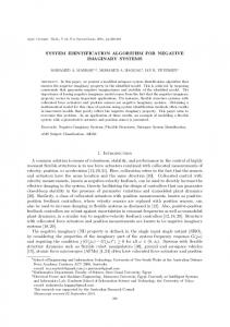
¡ ¢T with u(n) = u(n) · · · u(n − M + 1) . One can note that provided R ¿ M, the number of parameters can be significantly reduced from M 3 for the standard Volterra model to 3MR for the PARAFAC-Volterra model. However, the linearity in parameters is lost, the resulting model being trilinear in its parameters. Fig. 5 illustrates the parallel computation of the cubic PARAFAC-Volterra model output. ¡ ¢¡ ¢ By defining φrA (n) = uT (n)B.r uT (n)C.r , we can rewrite (26) as:   A.1 R ¡ ¢   y(n) ˆ = ∑ φrA (n)uT (n)A.r = φ1A (n)uT (n) · · · φRA (n)uT (n)  ...  r=1 A.R = vTA (n)vec(A),

(27)

¡ ¢T where vA (n) = φ A (n) ⊗ u(n) and φ A (n) = φ1A (n) · · · φRA (n) . Similarly, we get: y(n) ˆ = vTB (n)vec(B) = vCT (n)vec(C), (28) with ¡ ¢T vB (n) = φ B (n) ⊗ u(n), φ B (n) = φ1B (n) · · · φRB (n) , ¡ ¢¡ ¢ φrB (n) = uT (n)A.r uT (n)C.r , ¡ ¢T vC (n) = φ C (n) ⊗ u(n), φ C (n) = φ1C (n) · · · φRC (n) , ¡ ¢¡ ¢ φrC (n) = uT (n)A.r uT (n)B.r .

! "#

$ %&

#" ''( 9

A.1 B.1

X

C.1 u(n)

. . .

^y(n) +

A.R B.R

X

C.R

Fig. 1. Parallel realization of a cubic PARAFAC-Volterra model.

−

( 10

Now, we consider a linearization around the current estimates of two matrix components, and we define three conditional LS cost functions: n ¡ ¢2 ηX (n) = ∑ λ n−t y(t) − vˆ TX (n/n − 1)vec(X) , with X = A, B, C,

(29)

t=1

where λ is a forgetting factor, vˆ A (n/n − 1), vˆ B (n/n − 1), and vˆ C (n/n − 1) deˆ − 1)) , (A(n), ˆ ˆ − 1)), and (A(n), ˆ ˆ − 1), C(n ˆ pend respectively on (B(n C(n B(n)). By alternatively minimizing these cost functions with respect to A, B, and C, we get the following alternating recursive least squares (ARLS) algorithm: ˆ ˆ − 1)) + εX (n)kX (n) vec(X(n)) = vec(X(n

(30)

ˆ − 1)) εX (n) = y(n) − vˆ TX (n/n − 1)vec(X(n QX (n − 1)ˆvX (n/n − 1) kX (n) = T 1 + vˆ X (n/n − 1)QX (n − 1)ˆvX (n/n − 1) ¡ ¢ QX (n) = λ −1 I − kX (n)ˆvTX (n/n − 1) QX (n − 1).

(31)

with

(32) (33)

The ARLS algorithm can be summarized as follows: ˆ ˆ ˆ 1. Initialize B(0) and C(0) with random values, A(0) = 0, and QA (0) = QB (0) = QC (0) = α IMR , where α is a large arbitrary constant. Set n = 0. 2. Update the PARAFAC matrix factors: (a) Increment n. (b) Update of matrix factor A: i. Compute vˆ A (n/n − 1). ˆ ii. Compute A(n) using (30)-(33). (c) Update of matrix factor B: i. Compute vˆ B (n/n − 1). ˆ ii. Compute B(n) using (30)-(33). (d) Update of matrix factor C: i. Compute vˆ C (n/n − 1). ˆ ii. Compute C(n) using (30)-(33). 3. Go back to step 2 until convergence of the algorithm. 4. Reconstruct the Volterra kernel with the estimated PARAFAC loading factors: hˆ 3 (i1 − 1, i2 − 1, i3 − 1) =

R

∑ aˆi1 ,r bˆ i2 ,r cˆi3 ,r .

r=1

! "#

%& *

'' 11

4

Supervised identification of Wiener-Hammerstein systems [8].

Let us consider the Wiener-Hammerstein system depicted in Fig. 2.

Fig. 2. Wiener-Hammerstein system

Assuming that the nonlinearity is continuous within the considered dynamic range, then, owing to the Weierstrass theorem, it can be approximated to an arbitrary degree of accuracy by a polynomial C(.) of finite degree P, with coefficients c p . So, the WH model is composed of a polynomial C(.), sandwiched between two linear filters with impulse responses l(.) and g(.), and memories Ml and Mg respectively, i.e.: Ml −1

v1 (n) =

∑

P

l(i)u(n − i), v2 (n) =

i=0

∑ c p v1p (n),

p=1

Mg −1

y(n) =

∑

g(i)v2 (n − i),

(34)

i=0

with l(0) = g(0) = 1, a standard constraint for guaranteing the model uniqueness. The estimation of the parameters that characterize each block of this model is not simple since this model is not linear in its parameters. This parameter estimation problem can be solved by first identifying an associated Volterra model, linear in its parameters, and then deducing the parameters of linear and nonlinear subsystems from the estimated Volterra kernels. Several methods based on this approach were proposed by considering first- and second-order Volterra kernels in time [9] or frequency[10–12] domain.

− 12

The output of the Volterra model associated with the Wiener-Hammerstein system represented by means of equations (34) can be written as P

y(n) =

Mv

∑ ∑

p=1 i1 ,··· ,i p =1

p

h p (i1 − 1, · · · , i p − 1) ∏ u(n − ik + 1)

(35)

k=1

where h p (.), denoting the pth-order Volterra kernel associated with the WH system, is given by [13]: Mg

p

i=1

k=1

h p (i1 − 1, · · · , i p − 1) = c p ∑ g(i − 1) ∏ l(ik − i),

(36)

i = 1, · · · , Mg , ik = 1, · · · , Mv , k = 1, · · · , p, with Mv = Ml + Mg − 1. The Wiener-Hammerstein structure can be used for modelling communication channels where nonlinearities are structured as combinations of dynamic linear time-invariant (LTI) blocks with zero-memory nonlinear (ZMNL) ones. It finds application for modelling distortions in nonlinearly amplified digital communication signals (satellite and microwave links), among others. In the sequel, we consider a nonlinear communication channel represented with a WH model where the nonlinearity is due to the presence of a High Power Amplifier (HPA) at the transmitter of a mobile communication system. The linear filters l(.) and g(.) respectively characterize the transmit filter and the propagation bandpass channel whereas the memoryless nonlinear part C(.) represents the zero-memory HPA. It has been shown that the equivalent baseband representation of the ZMNL-HPA contains only odd-order terms [14, 15]: P

v2 (n) = C(v1 (n)) =

∑ α2p+1 [v1 (n)] p+1 [v∗1 (n)] p ,

(37)

p=0 Ml −1

where v1 (n) = ∑ l(i)u(n − i), u(.) being the input sequence. The received i=0

sequence y(.) is given by Mg −1

y(n) =

∑

g(i)v2 (n − i).

i=0

One can note that this representation is not linear with respect to the system parameters. So, parameter estimation of such a system is not a trivial task. However, this system also admits a Volterra model, linear-in-parameters and given

! "#

%& *

'' 13

by [16, 17]: P

y(n) =

∑

M−1

∑

p=0 i1 ,··· ,i2p+1 =0

p+1

2p+1

k=1

k=p+2

h2p+1 (i1 , · · · , i2p+1 ) ∏ u(n − ik )

∏

u∗ (n − ik )(38)

where M = Mg +Ml −1 and h2p+1 (., · · · , .) denotes the (2p+1)th-order Volterra kernel. Estimators devoted to linear models can easily be applied to the Volterra model. Since we are interested with the estimation of each subsystem, once the Volterra kernels estimated, we can deduce the parameters of both linear and nonlinear subsystems. Indeed, the Volterra kernels and the parameters of the original Wiener-Hammerstein model are linked as follows [18]: Mg −1

h2p+1 (i1 , · · · , i2p+1 ) = α2p+1

∑

i=0

p+1

2p+1

k=1

k=p+2

g(i) ∏ l(ik − i)

∏

l ∗ (ik − i).

(39)

In particular, the third-order Volterra kernel is given by: Mg −1

h3 (i1 , i2 , i3 ) = α3

∑

g(i)l(i1 − i)l(i2 − i)l ∗ (i3 − i)

i=0

or equivalently Mg

h3 (i1 − 1, i2 − 1, i3 − 1) = ∑ ai1 ,i bi2 ,i ci3 ,i ,

(40)

i=1

with ai1 ,i = α3 g(i−1)l(i1 −i), bi2 ,i = l(i2 −i), and ci3 ,i = l ∗ (i3 −i), i = 1, · · · , Mg , ik = 1, · · · , M, k = 1, 2, 3. We recognize in (40) the scalar writing of the PARAFAC decomposition of the M × M × M tensor H3 the elements of which are the coefficients of the thirdorder Volterra kernel h3 (.). The number of factors involved in this decomposition is equal to the memory Mg of the second linear subsystem. The three matrix factors A, B, and C, with the respective entries ai1 ,i , bi2 ,i , and ci3 ,i , are given by: A = Ldiag(γ ), B = L, C = L∗ ,

(41)

¡ ¢T with γ = α3 g, g = g(0) · · · g(Mg − 1) , L = T (l) the M × Mg Toeplitz ma¡ ¢T trix whose first column and row are respectively L.1 = lT 01×(Mg −1) and ¡ ¢ ¡ ¢T L1. = l(0) 01×(Mg −1) , and l = l(0) · · · l(Ml − 1) . In the sequel, we assume

−

$ 14

that l(0) = g(0) = 1. Assuming that the matrix factors fulfill the Kruskal condition, then the PARAFAC decomposition is essentially unique. Moreover, by taking the Toeplitz structure of L into account, with l(0) = 1, we can remove all column scaling and permutation ambiguities, so that the PARAFAC decomposition of the third-order Volterra kernel associated with a LTI-ZMNL-LTI system be strictly unique. Applying the formulae (3) with the correspondencies (41) and using the relation (2), we get the following M 2 × M unfolded matrices: H1 = (L∗ ¯ L) diag(γ )LT , H2 = (L ¯ L) diag(γ )LH ,

(43)

H3 = (L ¯ L∗ ) diag(γ )LT .

(44)

(42)

The parameters of the linear subsystems can be estimated using a two-step alternating least squares algorithm based on the minimization of the LS criterion ° °2 J = °H3 − (L ¯ L∗ ) diag(γ )LT °F . (45) Using the relation (1), this criterion can be rewritten as: J = kvec(H3 ) − (L ¯ L ¯ L∗ ) γ k22 .

(46)

It follows that the LS update of γ conditionally to the previous estimate Lˆ is given by ¡ ¢† (47) γˆ = Lˆ ¯ Lˆ ¯ Lˆ ∗ vec(H3 ). Defining G = diag(γ ) (L ¯ L∗ )T , we have ¢ ¡ ¢ ¡ HT3 = LG = T (l)G.1 · · · T (l)G.M2 = T (G.1 )l · · · T (G.M 2 )l .

(48)

So, we can rewrite the criterion J as ° °2 J = °vec(HT3 ) − Γ l°2 ,

(49)

¡ ¢T with Γ = T (G.1 )T · · · T (G.M2 )T . The conditional least squares update of l given the previous estimate Γˆ is then given by ˆl = Γˆ † vec(HT3 ).

(50)

-

! "#

%& *

'' 15

Once the linear subsystems estimated the system model becomes linear in the unknown remaining parameters, i.e. those of the ZMNL subsystem. So, the LS algorithm can be used to complete the system estimation. The overall estimation method is summarized as follows: 1. From input-output measurements, estimate the third-order Volterra kernel associated with the block structured nonlinear system to be estimated and construct the unfolded matrix H3 . 2. Estimate the parameter vectors γ and l as follows: (a) k = 0, initialize ˆl0 with random values, except ˆl0 (1) = 1. (b) k = k + 1, ˆ k−1 = T (ˆlk−1 ) and compute (c) Build L ¡ ¢† γˆ k = Lˆ k−1 ¯ Lˆ k−1 ¯ Lˆ ∗k−1 vec(H3 ). ¡ ¢ ˆ k = diag(γˆ ) L ˆ k−1 ¯ L ˆ ∗ T , and then (d) Deduce G k k−1 ¡ ¢T Γˆ k = T (Gk )T · · · T (Gk 2 )T . .1

.M

† (e) Compute ˆlk = Γˆ k vec(HT3 ) and normalize it by dividing its entries by the first one. (f) Return to step 2b until a stop criterion is reached4 . (g) Deduce the parameters of the second linear subsystem by dividing the entries of γˆ k by the first one, i.e. γˆ k (1). 3. (a) Generate the signals u¯2p+1 (n), n = 1, · · · , N, p = 0, · · · , P, as follows M−1

u¯2p+1 (n) =

∑

i1 ,··· ,i2p+1 =0

p+1

2p+1

k=1

k=p+2

hˆ 2p+1 (i1 , · · · , i2p+1 ) ∏ u(n−ik ) Mg −1

p+1

2p+1

i=0

k=1

k=p+2

∏

u∗ (n−ik ),

ˆ k − i) ∏ lˆ∗ (ik − i), where with hˆ 2p+1 (i1 , · · · , i2p+1 ) = ∑ g(i) ˆ ∏ l(i ˆ are the estimated parameters obtained in step 2. g(.) ˆ and l(.) (b) Calculate the LS estimate of the polynomial coefficient vector c = ¡ ¢ ¯ † y, with y = y(1) · · · y(N) T , the vector of (α1 · · · α2P+1 )T as cˆ = U ¡ ¢T ¯ = u(1) ¯ ¯ · · · u(N) , and the measured outputs, U ¡ ¢T ¯ u(n) = u¯1 (n) · · · u¯2P+1 (n) . 4

The stop criterion can be a given number of iterations

−

) 16

The third-order Volterra kernel can be estimated using a closed-form expression like that derived for third and fifth order Volterra channels with i.i.d. QAM and PSK input signals [17]. For more general i.i.d. signals and real-valued Volterra kernels, the closed-form espressions derived in [19] can also be used. Now, we illustrate the above algorithm by means of simulations where the linear subsystems of the simulated LTI-ZMNL-LTI communication channel are given by l = (1, 1 + j, −1 + j)T and g = (1, 1.05 + 0.8 j)T respectively whereas the parameters of the ZMNL part are α1 = 14.9740 + 0.0519 j and α3 = −23.0954 + 4.9680 j, which correspond to the parameters of a class AB power amplifier [15]. The input signal was an i.i.d. √ ª i.e. drawn √ 8-QAM sequence, from the finite alphabet Λ = {±1 ± j , ±(1 + 3), ±(1 + 3) j , with length N = 16384. An additive, zero-mean, complex, white Gaussian noise was added to the system output. The simulation results were averaged over 100 independent Monte Carlo runs. The performances were evaluated in terms of Normalized Mean Square Error (NMSE) on the output signal and on the estimated parameters. The third-order Volterra kernel was estimated using the method described in [17]. Figure 3 depicts the convergence behavior of the proposed two-steps ALS algorithm in terms of the estimated parameters of the two linear subsystems and the reconstructed third-order Volterra kernel in the noiseless case. From these simulation results, we can conclude that the two-steps ALS converges fast (about 30 iterations). In the noisy case, Figure 4 depicts the NMSE for different SNR values. We can note that the output NMSE corresponds approximately to the noise level, implying that the estimated model well approximates the simulated system. We also note that the estimation performances of the two LTI subsystems are very close.

5

Conclusion

In this second part of the paper, some applications of the PARAFAC model have been presented for solving the system identification problem for both SISO and MIMO FIR linear systems and nonlinear Volterra and Wiener-Hammerstein systems. In the cases of FIR linear systems and nonlinear Wiener-Hammerstein systems, the PARAFAC modeling results from the original structure of the systems. In the case of nonlinear Volterra systems, the PARAFAC model is used for reducing the parametric complexity. In the three cases, the computation of

.

! "#

%& *

'' 17

5

10

Third−order Volterra kernel First linear subchannel Second linear subchannel

0

10

−5

10

NMSE

−10

10

−15

10

−20

10

−25

10

−30

10

0

20

40 60 Number of iterations

80

100

Fig. 3. ALS convergence for the noiseless LTI-ZMNL-LTI communication channel.

10 Output First linear subchannel Second linear subchannel ZMNL subchannel

0

NMSE (dB)

−10

−20

−30

−40

−50

−60

0

5

10

15 SNR (dB)

20

25

30

Fig. 4. Output NMSE and parameter NMSE for the estimated LTI-ZMNL-LTI communication channel.

− 18

the PARAFAC parameters has been carried out using the ALS algorithm. It is to be noticed that other algorithms could also be applied. For instance, an extended Kalman filter based solution has been derived for PARAFAC-Volterra models [20]. Recently, the authors have proposed a new tensor-based approach for structure identification of block-oriented nonlinear systems [21]. In conclusion, tensors are very well suited for system identification by means of HOSbased methods as well as for nonlinear system representation and their structure and parameter estimation.

References 1. Bendat, J.: Nonlinear system analysis and identification from random data. John Wiley & Sons (1990) 2. Kearney, R., Stein, R., Parameswaran, L.: Identification of intrinsic and reflex contributions to human ankle stiffness dynamics. IEEE Trans. on Biomedical Engineering 44(6) (1997) 493–504 3. Korenberg, M., Hunter, I.: The identification of nonlinear biological systems: LNL cascade models. Biological Cybernetics 55 (1986) 125–134 4. Feher, K.: Digital communications- Satellite/Earth station engineering. Englewood Cliffs NJ: Prentice Hall (1993) 5. Kalafatis, A., Wang, L., Cluett, W.: Identification of Wiener type nonlinear systems in a noisy environment. International Journal of Control 66(6) (1997) 923–941 6. Fernandes, C.E.R., Favier, G., Mota, J.C.M.: Blind channel identification algorithms based on the PARAFAC decomposition of cumulant tensors: the single and multiuser cases. Signal Processing 88(6) (2008) 1382–1401 7. Khouaja, A., Favier, G.: Identification of PARAFAC Volterra cubic models using an alternating recursive least squares algorithm. In: Proc. 12th European Signal Processing Conference (EUSIPCO), Vienna, Austria (2004) 1903–1906 8. Kibangou, A., Favier, G.: Matrix and tensor decompositions for identification of block-structured nonlinear channels in digital transmission systems. In: Proc. IEEE Signal Proc. Advances in Wireless Communications (SPAWC), Recife, Brazil (2008) 9. Haber, R.: Structural identification of quadratic block-oriented models. Int. J. Systems Science 20(8) (1989) 1355–1380 10. Weiss, M., Evans, C., Rees, D.: Identification of nonlinear cascade systems using paired multisine signals. IEEE Trans. on Instrum. and Measurement 47(1) (1998) 332–336 11. Vandersteen, G., Schoukens, J.: Measurement and identification of nonlinear systems consisting of linear dynamic blocks and one static nonlinearity. IEEE Trans. on Automatic Control 44(6) (1999) 1266–1271

! "#

%& *

'' 19

12. Hui Tan, A., Godfrey, K.: Identification of Wiener-Hammerstein models using linear interpolation in the frequency domain (LIFRED). IEEE Trans. on Instr. and Measurement 51(3) (2002) 509–521 13. Kibangou, A., Favier, G.: Wiener-Hammerstein systems modeling using diagonal Volterra kernels coefficients. IEEE Signal Proc. Letters 13(6) (2006) 381–384 14. Benedetto, S., Biglieri, E., Daffara, E.: Modeling and performance evaluation of nonlinear satellite links- a Volterra series approach. IEEE Trans. on Aerospace and Electronics Systems 15(4) (1979) 494–506 15. Tong Zhou, G., Raich, R.: Spectral analysis of polynomial nonlinearity with applications to RF power amplifiers. EURASIP Journal on Applied Signal Processing 12 (2004) 1831–1840 16. Tseng, C.H., Powers, E.: Identification of nonlinear channels in digital transmission systems. In: Proc. of IEEE Signal Processing Workshop on Higher-order Statistics, South Lake Tahoe, CA (1993) 42–45 17. Cheng, C.H., Powers, E.: Optimal Volterra kernel estimation algorithms for a nonlinear communication system for PSK and QAM inputs. IEEE Trans. on Signal Processing 49(1) (2001) 147–163 18. Prakriya, S., Hatzinakos, D.: Blind identification of linear subsystems of LTIZMNL-LTI models with cyclostationary inputs. IEEE Trans. on Signal Processing 45(8) (1997) 2023–2036 19. Kibangou, A., Favier, G.: Identification of fifth-order Volterra systems using I.I.D. inputs. IET Signal Processing (2009) To appear. 20. Favier, G., Bouilloc, T.: Identification de modèles de Volterra basée sur la décomposition PARAFAC. In: Proc. of GRETSI’09, Dijon, France (2009) 21. Kibangou, A., Favier, G.: Tensor-based identification of the structure of blockoriented nonlinear systems. In: Proc. IFAC Symp. on System Identification (SYSID), Saint Malo, France (2009)

−

(