Sep 12, 2016 - non-elliptic web with a single-cycle W and [B(W)] is obtained from [W] . ...... The signature of a web W, denoted by Ï, is defined as the word in ...
TENSOR DIAGRAMS AND CHEBYSHEV POLYNOMIALS
arXiv:1609.03501v1 [math.CO] 12 Sep 2016
LISA LAMBERTI Abstract. In this paper, we describe a class of elements in the ring of SL(V )-invariant polynomial functions on the space of configurations of vectors and linear forms of a 3dimensional vector space V. These elements are determined by Chebyshev polynomials of the first and second kind with coefficients. We also investigate the relation between these polynomials and Lusztig’s dual canonical basis in tensor products of representations of Uq (sl3 (C)).
Contents 1. Introduction 2. SL(V)- invariants and Chebyshev polynomials 3. The Uq (sl3 (C))-invariant space Inv(V ) 4. Alternative evaluation of monomial webs in Inv(V ) 5. Lusztig’s dual canonical basis for Inv(V ) 6. Red graphs 7. Chebyshev polynomials and Lusztig’s dual canonical basis References
1 9 18 24 27 28 31 36
1. Introduction Given a complex vector space V , consider the ring Ra,b (V ) = C[(V ∗ )a × V b ]SL(V ) of polynomial functions on the space of configurations of a vectors and b covectors which are invariant under the natural action of SL(V ). Rings of this type play a central role in representation theory, and their study dates back to Hilbert. Over the last three decades, bases of Ra,b (V ) with remarkable properties were found by Lusztig [33, 34] and independently by Kashiwara [24], and further studied by Kuperberg [27], Lusztig [35], Geiss-Schr¨oerLeclerc [21], Fontaine-Kremnitzer-Kuperberg [18], Gross-Hacking-Keel-Kontsevich [23]. To explicitly construct, as well as to compare, some of these bases remains a challenging problem, already open when V is 3-dimensional. New perspectives in the study of canonical bases for Ra,b (V ) were suggested by Fomin and Pylyavskyy [14] by establishing that Ra,b (V ) has (several) structures of cluster algebras, when V is 3-dimensional. These cluster algebra structures provide a way to determine canonical bases in Ra,b (V ) by comparison with other rings which are cluster algebras and possess the notion of dual canonical bases. In particular, the set of cluster monomials forms the dual canonical basis of Ra,b (V ) when a = 0 and b ≤ 8 and (conjecturally) a subset for all other values of a and b. To describe all dual canonical basis elements is an open problem already for R0,9 (V ). This project was supported by the SNF grant P2EZP2148747. 1
The main goal of this work is to exploit earlier results on canonical bases for cluster algebras associated to Riemann surfaces in order to show that there are SL(V )-invariants in Ra,b (V ) which can be described naturally by recursive operations with desirable positivity properties. The recursions we find are Chebyshev polynomials (of the first or second kind). For these polynomials we also provide a combinatorial description in the language of tensor diagrams. More precisely, we consider Chebyshev polynomials in invariants in Ra,b (V ) described by the simplest planar tensor diagrams which do not have a description as single tree diagrams. The approach we suggest is similar to the topological characterization of Chebyshev polynomials in surface cluster algebras [38] and skein algebras [42]. In the second part of this paper, we investigate the relation between the SL(V )invariants described by Chebyshev polynomials of the second kind and the dual of Lusztig’s canonical basis for the invariant space of tensor products of fundamental representations of Uq (sl3 (C)), denoted by Inv(V ) and defined in [33]. For this we exploit the graphical computations originating in work of [19, 25, 20] relating Lusztig’s dual canonical and Kuperberg’s web basis, as well as a more recent approach using the combinatorial tool of red graphs and Khovanov-Kuperberg algebras developed in [40] together with the decategorification of [36]. In particular, we consider the third and fifth Chebyshev polynomials of the second kind U3 ([W ], [B(W )]) and U5 ([W ], [B(W )]) where [W ] is described by the by smallest non-elliptic web with a single-cycle W and [B(W )] is obtained from [W ] . We then show that for at least one of these two polynomials, there is no dual canonical basis element with integer coefficients that specializes to U3 ([W ], [B(W )]) or U5 ([W ], [B(W )]) at q = 1. Connections between Chebyshev polynomials of the second kind and Lusztig’s dual canonical bases were first made explicit in [29] and in [3, 9, 28]. In these papers a deformation of the usual cluster algebra of Kronecker type was considered, in the sense of [2], arising as a subalgebra of the positive part Uq (n) of the universal enveloping al(1) gebra of a Kac-Moody Lie algebra of type A1 . In this situation, the specialization of Lusztig’s dual canonical basis [32], at the classical limit at q = 1, is given by the set of all cluster monomials together with Chebyshev polynomials of the second kind in one variable parametrized by the imaginary root in the corresponding root system. Moreover, the quadratic Chebyshev polynomial of the second kind, U2 ([W ], [B(W )]), for [W ] and [B(W )] as before, is a dual canonical basis element in Inv(V ), as shown in [25]. On the other side, connections between Chebyshev polynomials of the first kind and Lusztig’s semi canonical basis [35] were made explicit in [29] and [21, 18]. Chebyshev polynomials and cluster algebras were first related to each other in the work of Sherman and Zelevinsky [41] where linear bases for rank 2 cluster algebras of affine types with certain nice properties were constructed. Since then Chebyshev polynomials have been linked to cluster combinatorics in several important contexts: • • • •
Bases for surface cluster algebras and skein algebras [41, 42, 38, 6, 37]. Canonical bases of cluster varieties related to SL2 local systems [13]. Theta/greedy bases for rank 2 cluster algebras [23, 8, 31, 30]. Quiver representation theory [29, 5, 12, 11, 10].
2
1 3!
[thick3 (W )] = [W ]3
[brac3 (W )]
P
σ
σ∈S3
[band3 (W )]
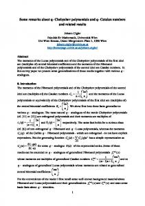
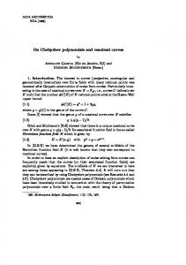
Figure 1. Tensor diagrams defining the invariants [W ]3 , [brac3 (W )] and [band3 (W )] of the single-cycle web W of lengths six, in red in the Figure. Our study of Chebyshev polynomials (of the first or second kind) in Ra,b (V ) should prove useful whenever one needs to recognize and distinguish different “canonical” bases of Ra,b (V ) and quantizations thereof. 1.1. Commutative case. Let V be a 3-dimensional complex vector space and let V ∗ = HomC (V, C) be the dual space. Let X = (V ∗ )a × V b be the direct product of a-copies of V ∗ and b-copies of V for a, b ∈ N. The special linear group SL(V) naturally acts on X and on its coordinate ring C[X]. Let Ra,b (V ) = C[X]SL(V) be the commutative associative ring of SL(V)-invariant polynomials on X. Many important invariants in Ra,b (V ) can be described graphically in terms of tensor diagrams. These are finite bipartite graphs with a fixed proper coloring of their vertices in two colors, black and white, and with a fixed partition of their vertices into boundary and internal vertices. Each internal vertex of a tensor diagram D is trivalent and comes with a fixed cyclic order of the edges incident to it. If the boundary of D consists of a white vertices and b black ones, one says that D has type (a, b). The coloring of the boundary of D determines a binary cyclic word, called signature of D. Moreover, each invariant of Ra,b (V ) can be described uniquely by a C-linear combination of invariants associated with non-elliptic webs. These are planar tensor diagrams such that all interior faces have at least six sides. The C-linear basis spanned by invariant defined by non-elliptic webs is Kuperberg’s web basis [27]. Let [W ] be the invariant in Ra,b (V ) defined by an arbitrary non-elliptic web W of type (a, b) with a single internal cycle and no four cycles (in particular this excludes that W has a quadrilateral with one vertex on the boundary attached to its internal cycle). In this paper we consider three operations applied on [W ]. The first operation is the ordinary power, represented in [14] by superimposing k-copies of W . The invariant described in this way, can be expressed in Kuperberg’s web basis by a single non-elliptic web invariant called the k-thickening of W , denoted by [thickk (W )]. The second operation is the k-bracelet operation, denoted by [brack (W )] and represented by concatenating k copies of W in such a way that the resulting tensor diagram sits on a M¨obius strip. The third operation is the k-band operation, denoted by [bandk (W )], represented by averaging over all possible ways of joining k copies of W , placed on top of each other For each of these operations, we bundle together k-tuples of adjacent identically colored endpoints coming from the k-copies of W . These operations are illustrated in Figure 1 for [W ] defined by the minimal single-cycle web W drawn in red on the left of the figure. We give formulas for invariants associated to the bracelet and band operation of [W ]. To state these results, we introduce the invariant [B(W )] = 12 ([W ]2 − [brac2 (W )]) defined 3
=
[B(W )]
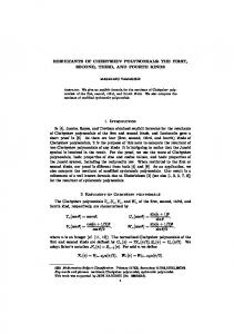
[W ]
Figure 2. Tensor diagrams defining the invariant [B(W )] associated to the invariant [W ] on the left. by a tensor diagram B(W ) obtained from W . For every single-cycle non-elliptic web W , the tensor diagram B(W ) can always be described as a single non-elliptic web, or equivalently as a superimposition of some tree diagrams. In Figure 2 we illustrate the two tensor diagrams defining [B(W )] corresponding to [W ] described by the non-elliptic web on the left hand side. Theorem 1.1. The k-bracelet operation of W is given by [brack (W )] = Tk ([W ], [B(W )]) where Tk (x, y) is the rescaled Chebyshev polynomial of the first kind defined by the recurrence T0 (x, y) = 2, T1 (x, y) = x, Tk (x, y) = xTk−1 (x, y) − yTk−2 (x, y). Recall that the usual Chebyshev polynomials of the first kind Chebk (x) are defined by Chebk (cos x) = cos(kx), k ∈ Z≥0 . The polynomials Tk (x, y) are related to these by Tk (x, y) = 2Chebk ( 2√x y )y k/2 Theorem 1.2. The k-band operation of W is given by [bandk (W )] = Uk ([W ], [B(W )]) where Uk (x, y) is the rescaled Chebyshev polynomial of the second kind defined by the recurrence U0 (x, y) = 1, U1 (x, y) = x, Uk (x, y) = xUk−1 (x, y) − yUk−2(x, y). d Tk (x, y) = kUk−1 (x, y). Hence, The polynomials Uk (x, y) are related to Tk (x, y) by dx � d x k/2 kUk−1 (x, y) = dx 2Chebk ( 2√y )y . As a corollary of these results, we show that the ordinary k-power [W ]k can be expressed as a positive integer linear combination of invariants associated to the band, resp. bracelet operation of [W ]. This contrasts with expanding [brack (W )], resp. [bandk (W )], in the web basis, where one uses the polynomials Tk ([W ], [B(W )]), resp. Uk ([W ], [B(W )]), which have negative coefficients. We next explain how Theorem 1.1 and Theorem 1.2 relate to previous work.
4
1.2. The cluster algebra of Kronecker type. Let F = Q(x1 , x2 ) be the field of rational functions in two commutating independent variables x1 and x2 with rational coefficients. Recursively define xj ∈ F by xj−1 xj+1 = x2j + 1. Consider the subring of F (1) generated by all xj , j ∈ Z, subject to the above relation. This subring, denoted by A1 , is an example of a coefficient free cluster algebra [16]. The generators are the cluster variables and the relation is called exchange relation. The sets {xj , xj+1 }, for j ∈ Z, are clusters and an element of the form xkj xlj+1 , for k, l ∈ Z≥0 , is called a cluster monomial. (1) This cluster algebra is of rank 2 and corresponds to the root system of affine type A1 , and therefore called of Kronecker type. (1)
Following [41], we now recall three distinguished natural bases for A1 . The topological description of these bases leads to the three operations we consider in Ra,b (V ). (1) Consider the distinguished variable z = x0 x3 − x1 x2 ∈ A1 expressed in {x0 , x1 } and {x2 , x3 }. Let the Chebyshev polynomials of the first kind in this variable, Tk (z), for k ≥ 1, be defined by the same recursion as before, when setting y = 1. Theorem 1.3. [41, Thm. 2.8] The disjoint union of the set of all cluster monomials and (1) the set {Tk (z)|k ≥ 1} is a Z-linear basis of A1 . This basis is the greedy basis in [31], which we now know coincides with the theta basis of [23], as shown in [8]. (1) To introduce the second basis for A1 consider the family of Chebyshev polynomials of the second kind Uk (z), k ≥ 1, in the same variable z as above. Theorem 1.4. [5] The disjoint union of the set of all cluster monomials and the set (1) {Uk (z)|k ≥ 1} is a Z-linear basis of A1 . This basis was called semicanonical in [5, 43] but later turned out to coincide with the specialization of Lusztig’s dual canonical basis at q = 1, see [9, 28]. (1) The third basis for A1 is the standard monomial basis, described in bigger generality in [1], and here given by {y0a0 y1a1 y2a2 y3a3 : am ∈ Z≥0 , a0 a2 = a1 a3 = 0} (1)
where y0 , y1, y2 , y3 are any four consecutive cluster variables of A1 . Unlike the previous two, the standard monomial basis is the one with fewer canonical properties. (1)
Topologically, the combinatorics governing A1 can be described through (isotopy classes of) arcs inside an annulus with one marked point on each boundary component. In this approach, the variable z is parametrized by the closed loop in the interior of the annulus, denoted δ. The polynomials Tk (z) can then be described by the k-bracelet operation on δ. That is, by superimposing k-copies of δ and forming a (k − 1)-self crossing. Similarly, the polynomials Uk (z) can be described by the k-band operation on δ. That is, by averaging over all possible ways of joining parallel k-copies of δ. The last operation is the specialization of standard Jones-Wenzl idempotents, also called magic elements, at q = 1, see also Remark 4.22 in [42]. Much of this was later generalized to cluster algebras associated to compact oriented Riemann surfaces [15] (possibly with boundary) by [38] and to surface skein algebras in [42]. In these settings, Chebyshev polynomials of the first, resp. second, kind are taken in the variables associated to all closed non-contractible curves in the surface, and can 5
be described again by the bracelet, resp. band, operations on these loops. The three operations defined in the setting of tensor diagrams in this paper, are generalizations of these operations for non-contractible curves. Moreover, our Theorem 1.1 and Theorem 1.2 can be seen as partial results towards finding bases for Ra,b (V ), generalizing Theorem 1.3, resp. Theorem 1.4. To extend the union of the disjoint sets of all cluster monomials and Chebyshev polynomials of the first, resp. second kind, in all single-cycle non-elliptic web invariants to bases of Ra,b (V ) remains an open problem. 1.3. Non-commutative case. We begin recalling the basic set up from [25]. Let Uq (sl3 (C)) be the quantum group corresponding to the Lie algebra sl3 (C). We follow the convention of setting v = −q 1/2 and view Uq (sl3 (C)) as an associative Hopf algebra over C(v). Let V ◦ and V • be the two 3-dimensional irreducible representations of type I of Uq (sl3 (C)) specializing to V and V ∗ when q → 1. Let S = (s1 , s2 , . . . , sn ) ∈ {◦, •}n be an arbitrary signature and consider the tensor product of irreducible representations V S = V s1 ⊗ V s2 · · · ⊗ V sn . This tensor product will be turned again into a representation of Uq (sl3 (C)) and we will consider the space of invariants: Inv(V S ) = {e ∈ V S : Y · e = ǫ(Y )e for all Y ∈ Uq (sl3 (C))} where ǫ : Uq (sl3 (C)) → C(v) is the counit of Uq (sl3 (C)) defined on the standard generators of Uq (sl3 (C)) by: ǫ(Ei ) = ǫ(Fi ) = 0 ǫ(Ki ) = 1. The vector space of all invariants is denoted by Inv(V ). This space is of particular interest to us for the following reasons. • For any signature S the dual canonical basis has been defined in Inv(V S ) and hence in Inv(V ). This basis is dual to the canonical basis defined by Lusztig’s [33] and related to the global crystal basis of Kashiwara [24] independently defined also in [32]. • At the classical limit the invariant space Inv(V ) specializes to the polynomial invariant ring Ra,b (V ), as we explain later. • The quadratic Chebyshev polynomial of the second kind in the invariant defined by the smallest single-cycle web belongs to Lusztig’s dual canonical basis for Inv(V ), see see [25, Thm. 4]. More precisely, Kuperberg’s web basis extends to a C(v)-linear basis for Inv(V ). The relationship between the web basis and Lusztig’s dual canonical basis of Inv(V ) was investigated by Khovanov and Kuperberg [25]. They discovered that these two bases are in general different from each other, despite despite overlapping substantially and sharing several properties. To describe the discrepancy they found, in the language of this paper, consider again the non-elliptic webs defining the invariants [thickk (W )], [brack (W )], and [bandk (W )]. Different invariants, which we denote by [Thickk (W )], [Brack (W )], and [Bandk (W )] can be obtained from [thickk (W )], [brack (W )], and [bandk (W )] after splitting all endpoints of the non-elliptic webs defining the invariants [thickk (W )], [brack (W )], and [bandk (W )]. In Ra,b (V ) this splitting procedure represents the polarization of the corresponding invariant tensor. Khovanov and Kuperberg show that when W is the smallest single-cycle web, the web basis element [Thick2 (W )] does not lie in Lusztig’s dual canonical basis; instead, the element [Band2 (W )] is a dual canonical basis element, see [25]. It is then natural to 6
ask: do all invariants [Bandk (W )], k ∈ Z≥0 , belong to the specialization of Lusztig’s dual canonical basis at q = 1?
−
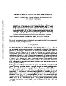
[B(W )]
[Band2 (W )]
[Band1 (W )] = [W ]
Figure 3. Three Lusztig’s dual canonical basis elements of Inv(V ) expressed in Kuperberg’s web basis. We give a negative answer to this question, when the coefficients of the dual canonical basis element are assumed to be integers. Proposition 1.5. Let W be the minimal single-cycle non-elliptic web. There is no Lusztig’s dual canonical basis element of Inv(V ) with integer coefficients that specializes to [Band3 (W )] or [Band5 (W )] when q → 1. The general case, in which coefficients involving q are allowed, remains open. In the middle of Figure 3, the minimal single-cycle non-elliptic web W is shown. It can be seen that the invariant [W ] ∈ Ra,b (V ) defined by this W plays the same role as the loop circling the annulus plays in the cluster algebra of Kronecker type discussed in Section 1.2. In fact, [W ] decomposes as z0 z3 −z1 z2 for the cluster variables in {z0 , z1 } and {z2 , z3 } belonging to a cluster subalgebra of Ra,b (V ) of Kronecker type, up to coefficients. 1.4. From Inv(V ) back to Ra,b (V ). Let X = (V ∗ )a × V b . Every polynomial in C[X] decomposes in a unique way into a sum of multihomogeneous functions Moreover, if a polynomial is SL(V )-invariant then every multihomogeneous function is also SL(V )invariant. Hence Ra,b (V ) decomposes as follows: MM SL(V ) C[X][p,q] . Ra,b (V ) = C[X]SL(V ) = p∈Na q∈Nb
To relate this space to the specialization of Inv(V ) at the classical limit we need to give another description of Ra,b (V ). For this let p ∈ Na and q ∈ Nb and consider (V ∗ )⊗p ⊗ V ⊗q = V ∗⊗p1 ⊗ · · · ⊗ V ∗⊗pa ⊗ V ⊗q1 ⊗ · · · ⊗ V ⊗qb . Then SL(V ) acts on V by the regular representation and on V ∗ by the Pdual representation. P Hence (V ∗ )⊗p ⊗ V ⊗q can be seen as a SL(V )-module. Let |p| = pi and |q| = qi . Let Sp = Sp1 × Sp2 × · · · × Spa acting as a group of permutations of {1, . . . , |p|}, where the symmetric group Sp1 permutes the factors in position 1 up to p1 , Sp2 permutes 7
p1 + 1, . . . , p1 + p2 , and so on. Then Sp × Sq acts on (V ∗ )⊗p ⊗ V ⊗q and the actions of Sp × Sq and SL(V ) commute. One then deduces: M Mh �Sp ×Sq iSL(V ) Ra,b (V ) ∼ (V ∗ )⊗|p| ⊗ V ⊗|q| = p∈Na q∈Nb
∼ =
M Mh
∗ ⊗|p|
(V )
p∈Na q∈Nb
⊂
MM
⊗V
iSp ×Sq � ⊗|q| SL(V )
(V ∗ )⊗|p| ⊗ V ⊗|q|
p∈Na q∈Nb
∼ = InvSL(V ) (V )
�SL(V )
where the first two lines are [22, Lemma 5.4.1]. One concludes observing that Inv(V ) specializes to InvSL(V ) (V ) when q → 1. Notice that the product in Inv(V ) is represented by disjoint union of tensor diagrams while the product in Ra,b (V ), being commutative, can be represented by superimposing the corresponding tensor diagrams (and clasping endpoints). 1.5. The quantum cluster algebra of Kronecker type. The rank 2 cluster algebra (1) of Kronecker type A1 associated to the annulus with one marked point on each boundary component deforms to a non-commutative quantum cluster algebra, in the sense of [2]. This quantum cluster algebra is a subalgebra of the positive part of the Kac-Moody Lie (1) algebra of type A1 . Moreover, this quantum cluster algebra is equipped with Lusztig’s canonical basis for quantized enveloping algebras [32] and its dual basis. This notion of dual canonical basis is different then the Lusztig’s notion for Inv(V ), considered in this paper, but closely related, as explained in [33]. (1) For the variable z = x0 x3 − x1 x2 ∈ A1 expressed in the cluster variables of {x0 , x1 } and {x2 , x3 } described before, the following two results are known. Theorem 1.6. [21] The disjoint union of the set of all cluster monomials and the set (1) {Tk (z)|k ≥ 1} belongs to the specialization of Lusztig’s semi canonical basis for A1 at q = 1. Theorem 1.7. [9] The disjoint union of the set of all cluster monomials and the set (1) {Uk (z)|k ≥ 1} belongs to the specialization of Lusztig’s dual canonical basis for A1 at q = 1. The last result also follows from work of Lampe [28] setting trivial coefficients, see also [3, 2]. 1.6. Two-dimensional case. In this setting Ra,b (V ) ∼ = R0,a+b (V ) ∼ = C[Gr2,a+b (C)]. It is well known that this ring is a cluster algebra corresponding to the root system of type An , and that set of all cluster monomials is a linear basis for C[Gr2,a+b (C)], see [17]. On the other side, Kuperberg’s web basis in the 2-dimensional case consists of non crossing matchings in a disc with marked points on the boundary, see [27, §.2]. If one divides the boundary points into a + b intervals and avoids U turns between endpoints in the same interval, as for clasped web spaces defined in [27, §. 2.2], one can see that Kuperberg’s web bases and the cluster monomial bases coincide. Moreover, these bases are known to be the specialization of Lusztig’s dual canonical bases for the invariant space in the tensor product of Uq (sl2 (C))-representations, see [19]. 8
In particular, it follows, that in the 2-dimensional setting there no Chebyshev polynomials occur in these bases. On the other extreme, extending the web-based approach to higher dimensions remains a major outstanding problem, since the concept of the web basis has no known natural generalization for vector spaces V of dimension 4 or greater. 1.7. General plan of the paper. In Section 2 we introduce the basic notions related to the commutative polynomial ring Ra,b (V ). We define the bracelet and band operations and prove Theorem 1.1 and Theorem 1.2. Properties of bases of Ra,b (V ) including [bandk (W )], resp. [brack (W )] as basis elements will also be discussed. Some of the results in this section already appeared in my PhD thesis. In Section 3 we pass to the non-commutative setting and describe the quantized tensor invariant space Inv(V ) algebraically and using tensor diagrams. The combinatorial methods of flows developed in [25] will also be revised in this section and we recall how invariants associated to non-elliptic web expand in the tensor product basis. In Section 4 we give an alternative description of the coefficients appearing in the decomposition in the tensor product basis of a collection of web invariants in Inv(V ), using only the boundary data of the non-elliptic web. In Section 5 we describe Lusztig’s dual canonical bases for Inv(V ). Following [25], we recall how Lusztig’s dual canonical bases relate to Kuperberg’s web bases for Inv(V ) and give a simple operation on non-elliptic web invariants preserving the property of being dual canonical. In Section 6 we review the definition of red graphs introduced in [40] and express in the language used in this paper some key results of [40] and [36]. In Section 7 we provide some preliminary results and prove Proposition 1.5. We conclude this section formulating further possible directions of investigation in Conjecture 7.8. 1.8. Acknowledgments. I would like to thank S. Fomin and P. Pylyavskyy for introducing me to this beautiful subject during the workshop on cluster algebras at MSRI, Berkeley, in 2012. I thank both of them for the always interesting and stimulating discussions we had since then. I also thank the Department of Mathematics of the University of Michigan for its hospitality and support during my research stay here. 2. SL(V)- invariants and Chebyshev polynomials We begin recalling some preliminary definitions and results following mainly [14]. Let V = C3 , and V ∗ = HomC (V 3 , C). Elements in V are vectors, while elements in V ∗ are convectors. Let ∗ X=V · · × V }∗ × V · · × V} . | × ·{z | × ·{z a−times
b−times
A tensor T of type (a, b) is a multilinear map T : X → C. Let vol : V 3 → C be the volume tensor with evaluation vol(v1 , v2 , v3 ) given by the oriented volume of the parallelotope with sides v1 , v2 , v3 . Let vol∗ : V ∗ 3 → C be the dual volume tensor defined by vol(v1 , v2 , v3 )vol∗ (u∗1 , u∗2, u∗3 ) = det(u∗j (vi )) 1≤i≤3 . 1≤j≤3
Let id : V ∗ × V → C be the identity tensor corresponding to the identity operator on V . Let e1 , e2 , e3 be the standard basis of V satisfying vol(e1 , e2 , e3 ) = 1, then vol∗ (e∗1 , e∗2 , e∗3 ) = 1. 9
Figure 4. Tensor diagrams associated to vol, vol∗ , and id. The action of the special linear group SL(V) on V induces a left action of SL(V) on V given by g · u∗ (v) = u∗ (g −1 · v) for g ∈ SL(V), v ∈ V and u∗ ∈ V ∗ . The action of SL(V) on X is given by g · (u∗ , v) = (g · u∗1 , . . . , g · u∗a , g · v1 , . . . , g · vb ) for g ∈ SL(V), (u∗ , v) = (u∗1 , . . . , u∗a , v1 , . . . , vb ) ∈ X. The action of SL(V) on the coordinate ring C[X] is given by (g · f )(u∗ , v) = f (g −1 · (u∗ , v)) for f ∈ C[X], g ∈ SL(V). ∗
Definition 2.1. Let Ra,b (V ) = C[X]SL(V) be the ring of SL(V)-invariant polynomials on X. A description of Ra,b (V ) in coordinate notation can be found in [14, Section 2]. The tensors vol, vol∗ and id are examples of SL(V)-invariant polynomials on X. Also Pl¨ ucker coordinates, dual Pl¨ ucker coordinates and bilinear forms obtained by paring covectors of V ∗ with vectors of V are SL(V)-invariant polynomials on X. By the First Fundamental Theorem of SL(V)-invariants Ra,b (V ) is generated by the last three types of tensors. To reflect the order of the covariant and contravariant arguments in Ra,b (V ) one associates to elements in Ra,b (V ) a word in the alphabet {◦, •} called signature. By convention the symbol ◦ represents covariant arguments, while • indicates the arguments of V . Then Rσ (V ) indicates the ring of SL(V)-invariants of signature σ. If σ consists of a copies of ◦ and b copies of • we say σ has type (a, b). It follows, that Rσ (V ) ∼ = Ra,b (V ) for σ of type (a, b). A handy way to express elements of Ra,b (V ) is given by tensor diagrams. Definition 2.2. A tensor diagram D is a finite bipartite graph with a fixed proper coloring of its vertices consisting of two colors, black and white, and with a fixed partition of its vertices into boundary and internal vertices. Each internal vertex of D is trivalent and comes with a fixed cyclic order of the edges incident to it. The edges of D might intersect transversally. If the boundary of D consists of a with vertices and b black ones, then D has type (a, b). Tensor diagrams, considered in this context, are build starting from the three building blocks associated to the tensors vol, vol∗ and id. More precisely, one represent the arguments of these tensors by arrows, so that sinks correspond to vectors and sources to covectors see Figure 4. To ensure that the tensor is well defined one also specifies a cyclic ordering of the corresponding three arguments. To obtain bigger tensors one then combines two such blocks by plugging arrowheads into arrow tails. This operation represents the contraction of the corresponding tensors. In the sequel, arrow sinks are replaced by black colored vertices, and arrow sources by white colored vertices. Moreover, tensor diagrams are drawn inside oriented discs, in such a way that the cyclic ordering of the edges incident to each interior vertex matches 10
the clockwise orientation of the disk and such that the endpoints of the tensor diagram lie on the boundary. Given an invariant [D] ∈ Ra,b (V ) one can substitute the same vector, or covector, into different arguments of [D]. This operation, called restitution, can be represented on tensor diagrams by boundary vertices having several incident edges. The inverse operation is called polarization. Gluing boundary points however does not preserve the multilinearity of the tensor. Given a tensor diagram D of type (a, b) an SL(V)-invariant [D] associated to D in Ra,b (V ) can be defined as follows: For each white vertex v of D let x(v) = (x1 (v), x2 (v), x3 (v))⊤ be the corresponding vector argument of the tensor associated to D, and for each black vertex v of D let y(v) = (y1 (v), y2(v), y3(v)) be the corresponding covector argument. The invariant [D] associated to D is given by [D] =
X� Y l
v∈int(D)
sign(l(v))
�� Y
v∈bd(D) vblack
x(v)l(v)
�� Y
v∈bd(D) vwhite
y(v)l(v)
�
where • The index l runs over all proper labellings of the edges of D by the numbers 1, 2, 3. Notice that for each internal vertex v of D the labellings of the three incident edges are all distinct; • sign(l(v)) is the sign of the cyclic permutation of those three labels determined by the cyclic ordering of the Q edges incident to v; l(v) • x(v) is the monomial e xl(e) (v), where e runs over all edges incident to v, similarly for y(v)l(v) . In [14, Example 4.2] this formula has explicitly been computed. Tensor diagrams naturally model the additive and multiplicative structure of Ra,b (V ). Multiplication is modeled using superimposition of diagrams. Notice that when D is a union of subdiagrams D1 , D2 , . . . connected only at the boundary vertices, then [D] = [D1 ][D2 ] . . . . Addition is obtained by allowing linear combinations of tensor diagrams and extending by linearity the definition of the invariant [D] associated to D. From the First Fundamental Theorem of invariant theory it follows that any SL(V)invariant of Ra,b (V ) can be written as a linear combinations of invariants associated to tensor diagrams constructed by superimposition of the building blocks corresponding to the vol and vol∗ tensors. This writing however is not unique. In Figure 5 a number of relations of invariants associated to tensor diagrams are illustrated. These relations, called skein relations for tensor diagrams, allow to transform a small fragment F of the diagram D into linear combinations of other diagrams F = ci Fi , ci ∈ N, where the Fi are tensor diagrams of the same type as F . Whenever the tensor P diagram corresponding to F defines the same invariant as ci Fi , one has that [D] = i ci [Di ], where Di indicates the tensor diagram obtained from D by replacing the fragment F with the other pieces Fi and keeping the rest of the diagram unchanged. The validity of the skein relations follow directly from the definition of tensors, see [4]. 11
(a) =
+
(b) +
= (c) (d)
=
2
=
3
(e) (f)
111 000 000 111
=
1111 0000 0000 1111
=0 =0
= 111 000
1111 0000
Figure 5 Definition 2.3. A web W is a tensor diagram embedded in an oriented disk so that its edges do not cross or touch each other, except at endpoints. Each web is considered up to isotopy of the disk that fixes its boundary. A web is non-elliptic if it has no multiple edges and no internal cycles of length less then or equal to four. The invariant [W ] associated to a non-elliptic web W is called a web invariant. The signature of a web W , denoted by σ, is defined as the word in the alphabet {◦, •} obtained from the boundary of W . Theorem 2.4 (Kuperberg [26]). Web invariants with a fixed signature σ of type (a, b) for a linear basis in the ring of invariants Rσ (V ) ∼ = Ra,b (V ). We now turn our attention to single-cycle webs and introduce different procedures to concatenate of copies of them. Definition 2.5. Let k be a positive integer, and let W be a non-elliptic web. The kthickening of W is obtained as follows: • replace each internal vertex of W by a “honeycomb” fragment Hk of the appropriated color, as shown in Figure 6(a); • replace each edge of W by a k-tuple of edges connecting the corresponding honeycombs and / or boundary vertices. In the sequel we denote the k-thickening of W by thickk (W ). Definition 2.6. A non-elliptic web with a single internal cycle of length at least six, is called a single-cycle web. A single-cycle web has alternating signature if adjacent boundary vertices are colored differently. For single-cycle webs W of arbitrary signature, one can find a single-cycle web S of alternating signature inside W . 12
00 11 00 11 11 00 00 0011 11 00 11 11 00 00 11 0 1 0 1 00 11 0 1 0 1 1 1 0 0 1 0 00 11 00 11 0 1 00 11 1 0 0 1 00 11 00 1 00 111 0 0 11 00 1 00 11 00 1 0 11 0 11 00 11
H1
H2
H3
H4
Figure 6. On the left honeycomb fragments are represented. On the right a single-cycle clasped web and its 2-thickening is represented.
Lemma 2.7. Let [W ] be the web invariant defined by a single-cycle web W of arbitrary signature. Then, each power [W ]k is a web invariant defined by thickk (W ). Proof. If W is a single-cycle web of alternating signature the result follows from skein relation (a) and (e). For more general single-cycle webs W, one finds a single-cycle web S contained in W of alternating signature. Let p be an internal vertex of W , which is an endpoint of S. Then there is a subtree W ′ of W attached to S in p. Concatenating k-copies of W one also superimposes k-copies of S, and k-copies of W ′ . Then W ′k = thickk (W ′) and S k is given by thickk (S) an terms which attach to the honeycomb fragments Hk of thickk (W ′ ). Recursively using skein relations (b), used from the interior of the diagram towards the boundary, yields the vanishing of the term. � In the following definitions, let k ∈ Z≥0 , and let W be a single-cycle web of arbitrary signature. Definition 2.8. The k-bracelet operation of W is the tensor diagram brack (W ) drawn on an oriented disk obtained by • superimposing k-copies of W creating k − 1-self crossings • gluing together the k-endpoints of the copies of W at the boundary of the disc. The k-bracelet operation is considered up to isotopy of the disc that fixes its boundary points. Definition 2.9. The k-band operation of W is the tensor diagram bandk (W ) drawn on an oriented disk obtained by • averaging over all possible ways of concatenating the internal cycles of k copies of W • gluing together the k-endpoints of the copies of W at the boundary of the disc. For convenience, band0 (W ) = 1 and brac0 (W ) = 2. In addition, bandk (D) = brack (D) = thickk (D) for every non-elliptic web D without any cycle (i.e. a planar tree tensor diagram). Remark 2.10. The bracelet and band operations can be used to detect ‘imaginary’ elements in Ra,b (V ). These are elements whose powers are not clasped web invariants, hence not expected to be cluster variables (c.f. Conjecture 9.3 in [14] and [29]). 13
We now recall some basic facts about the Chebyshev recursions, which we later link to the band and bracelet operation of single-cycle tensor diagrams. U0 (x, y) = 1
T0 (x, y) = 2
U1 (x, y) = x
T1 (x, y) = 1 T2 (x, y) = x − 2y
U2 (x, y) = x2 − y
T3 (x, y) = x3 − 3xy
U3 (x, y) = x3 − 2xy
T4 (x, y) = x4 − 4x2 y + 2y 2
U4 (x, y) = x4 − 3x2 y + y 2
T5 (x, y) = x5 − 5x3 y + 5xy 2 ...
U5 (x, y) = x5 − 4x3 y + 3xy 2 ...
2
Proposition 2.11. [38, Prop. 2.35] For all k ≥ 1, the monomial xk can be written as a positive integer linear combination of the Chebyshev polynomials Tk = Tk (x, y). In particular, � � � � k−1 k k yTk−2 + · · · + k−1 y 2 T1 , if k is odd; x = Tk + 1 � 2 � � � � � k−2 k k k k k yTk−2 + · · · + k−2 y 2 T2 + k y 2 T0 , if k is even. x = Tk + 1 2 2 k
Similarly, for Chebyshev polynomials of the second kind we deduce the following result. Proposition 2.12. For all k ≥ 1, the monomial xk can be written as a positive integer linear combination of the Chebyshev polynomials Uk = Uk (x, y). In particular, xk is given by (� � � (� � � �) �) k−1 k k k k − k−1 y 2 U1 yUk−2 + · · · + − Uk + k−1 −1 0 1 2 2 if k is odd; and by (� � � (� (� � � �) � � �) �) k−2 k k k k k k k − k y 2 U2 + y 2 U0 yUk−2 +· · ·+ − Uk + k − k k −1 −2 −1 0 1 2 2 2 2 if k is even. Proof. The positivity of the linear combination follows as the differences between binomial coefficients are taken between consecutive elements in the first half of the Pascal triangle. For the rest of the proof we proceed by cases, as for Chebyshev polynomials for the first kind, see [38, Prop. 2.35]. If k is odd, using the induction assumption, we have (� � � (� � � �) ! �) k−1 k k k k − k−1 y 2 U1 . yUk−2 + · · · + − x Uk + k−1 −1 0 1 2 2 14
Since xUk = Uk+1 + yUk−1, we rewrite xk+1 as (� � � (� � � �) ! �) k−1 k k k k − k−1 yUk−2 + · · · + y 2 U1 − x Uk + k−1 0 −1 1 2 2 (� � � (� � � �) �) k−1 k k k k − k−1 y 2 U2 yUk−1 + · · · + − =Uk+1 + k−1 −1 0 1 2 2 (� (� � � �) � � �) k−1 k k k k − k−1 y 2 U2 y 2 Uk−2 + · · · + − +y Uk−1 + k−1 −1 −2 0 1 2 2 (� � � ! ) � k+1 k k + − k−1 y 2 U0 . k−1 −1 2 2 For the coefficient of U0 we observe that � � � � � � k k 2 k+1 − k−1 = k−1 −1 k + 1 k−1 2 2 � � 2 2 k+1 = +1 k + 1 k+1 � �2 1 k+1 = k+1 + 1 k+1 2 2 � � � � k+1 k+1 = k+1 − k+1 . −1 2 2 We conclude using Pascal’s rule. If k is even, ! (� � � (� � � �) �) k k k k k k+1 yUk−2 + · · · + − − k y 2 U0 . x = x Uk + k 0 1 − 1 2 2 This is the same as (� � � (� � � �) �) k k k k k yUk−1 + · · · + − Uk+1 + − k y2x k 0 1 −1 2 2 (� (� � � �) � � �) k k k k k − k y 2 U1 . y 2Uk−3 + · · · + − + yUk−1 + k −1 −2 0 1 2 2 Observe that x = U1 , and conclude using Pascal’s rule.
�
As before, let W be a single-cycle web of arbitrary signature. We will now construct a non-elliptic web B(W ), associated to W . The invariant described by B(W ) will later play the role of the coefficient in the Chebyshev recursions. Definition 2.13. Let S be the single-cycle clasped web contained in W of alternating signature. Then B(W ) is obtained from thick2 (W ) by removing thick2 (S) in thick2 (W ) and joining the vertices formerly serving as endpoints of thick2 (S). As an example, the invariant [B(W )] obtained from thick2 (W ) as described above, for the single-cycle hexagonal non-elliptic web having a tripod attached at each end the, is illustrated in Figure 2. 15
Lemma 2.14. Let k be an integer. Let W be a single-cycle web of arbitrary signature. Assume that W has no quadrilateral with one vertex on the boundary attached to the internal single cycle. Then in the k-thickening of W the following local identities hold: (a) =
.. .
.. .
.. .
.. .
+
.. .
.. .
(b) .. .
.. .
= . ..
+
.. .
.. .
.. .
.. .
+. . .+
+
.. .
(c) .. .
= −2B(W ) ...
.. .
.. .
(d) .. .
.. + . . . + .
.. .
+
.. .
= B(W )
= B(W )
.. .
.. .
.. .
.. .
+ B(W )
.. .
Proof. Part (a) follows by solving the first crossing with the skein relation. Part (b) follows iteratively using skein relations on the first crossing. Part (c) follows by the multiplicative structure of tensor diagrams and skein relations. More precisely, since no quadrilateral with one vertex on the boundary attached to the internal single cycle, iteratively solving squares generates both new squares around the cycle as well as terms eventually vanishing (by skein relation (e)). The final collision of squares, around the internal cycle, produces the factor −2. By similar reasoning as in Part (c) we deduce the first equality in Part (d) observing that solving the upper square in the first summand of the expansion produces the first term on the right hand side of the equality. Solving the upper squares in the remaining summands, and summing the resulting terms, produces the second term, by the identity in Part (b). The second equality follows from Part (a) � Remark 2.15. If W has a quadrilateral with one vertex on the boundary attached to the internal single cycle then part (c) of the previous lemma leads to the vanishing of the corresponding invariant in Ra,b (V ). 16
Proof of Thm. 1.1. The initial condition T1 ([W ], [B(W )]) = [W ] is clear and a simple computation gives T2 ([W ], [B(W )]) = [W ]2 − 2[B(W )]. The recurrence then follows from Lemma 2.14 part (a) followed by part (b), (c) and (d). � Keeping the assumptions of Thm. 1.1 the next result can be deduced by Proposition 2.11. Corollary 2.16. The monomial [W ]k can be written by a positive linear combination of the Chebyshev polynomials of the first kind Tk = Tk ([W ], [B(W )]). In particular, � � � � k k k [B(W )](k−1)/2 T1 , if k is odd; [B(W )]Tk−2 + · · · + [W ] = Tk + (k − 1)/2 1 � � � � � � k k k (k−2)/2 k [B(W )]k/2 [B(W )] T2 + [B(W )]Tk−2 + · · · + [W ] = Tk + k/2 (k − 2)/2 1 if k is even. � Our coefficient [B(W )] in the expression for Chebyshev polynomials of the first kind is given by a product of coefficient variables for the given cluster algebra structure. To see this it suffices to remove the internal trivalent vertices of B(W ), using skein relations, and compare with Definition 6.1. in [14]. It follows that [B(W )] can be thought of as a generalization of the coefficient described in [38] associated to closed contractible curves in cluster algebras associated to 2-dimensional Riemann surfaces with non-empty boundary. Lemma 2.17. Let k be an integer. Let W be a single-cycle web of arbitrary signature. In the thickening of W the following local identities hold: (a) n
=
m
n
(b) n
=
n−1
1 n
=
n−1
n−1 +
+
n−1 n
n−1
n−1
n−1 n
n−1 (c) n n
=
=
n 17
n−1
+
n−1 n
n−1
Proof. The proof is a small adaptation of the surface case, treated in [42, Lemma 4.6]. The second equality in claim (b) follows from the skein relations in the thickening of a single cycle web and claim (a). The last claim follows from claim (b) and (a) and after having moving one box around the cycle using skein relations. � Proof of Thm. 1.2. Proceed by induction. For small n the claim can be checked directly. For n > 2, the claim can be deduce from Lemma 2.17 part (b), followed by part (c) and solving the squares in the two summands of part (c) following the reasoning of Lemma 2.14 parts (c) and (d). � Keeping the assumptions of Theorem 1.2 we deduce the next result with Proposition 2.12. Corollary 2.18. The monomial [W ]k can be written by a positive linear combination of the Chebyshev polynomials of the second kind Uk = Uk ([W ], [B(W )]). In particular, [W ]k is equal to (� � � (� � � �) �) k−1 k k k k [B(W )]Uk−2 + · · · + − Uk + − k−1 [B(W )] 2 U1 k−1 0 1 −1 2 2 if k is odd. Respectively, given by (� � � �) k k [B(W )]Uk−2 + · · · + − Uk + 0 1 (� � � (� � � �) �) k−2 k k k k k − k − k [B(W )] 2 U2 + [B(W )] 2 U0 k k −1 −2 −1 2 2 2 2 if k is even.
�
Remark 2.19. From the previous results we see that the expansion of [W ]k in the web basis uses Chebyshev polynomials Tk ([W ], [B(W )]), resp. Uk ([W ], [B(W )]), which have negative coefficients. However, [W ]k expands positively in bases containing Chebyshev polynomials Tk ([W ], [B(W )]), resp. Uk ([W ], [B(W )]), see Corollary 2.16 and Corollary 2.18. This matches with the expectations coming from the surface case, as described in remark 4.8 in [38]. Remark 2.20. A computation shows that the previous results also hold for more general web invariants defined by non-elliptic webs which arborize to tensor diagrams with a single internal cycle. An example of such a non-elliptic web together with it’s arborized form can be found at the bottom of Figure 31 in [14]. 3. The Uq (sl3 (C))-invariant space Inv(V ) In this section we follow [25] closely. Let C(q 1/2 ) be the field of complex-valued rational functions in the indeterminate q 1/2 . Let Uq (sl3 (C)) be the quantum group corresponding to the Lie algebra sl3 (C). Then Uq (sl3 (C)) is an associative algebra over C(q 1/2 ), with generators Ei , Fi , Ki and Ki−1 , 18
i = 1, 2, satisfying certain relations, see [25, §. 2]. Denote the quantum integer by [n] =
q n/2 − q −n/2 , q 1/2 − q −1/2
so for example [1] = 1, [2] = q 1/2 + q −1/2 , [3] = q + 1 + q. In the following, set v = −q 1/2 . A Hopf algebra structure on Uq (sl3 (C)) over C(v) can be defined setting up the coproduct ∆ as follows: ∆(Ki± ) = Ki± ⊗ Ki± ∆(Ei ) = Ei ⊗ 1 + Ki−1 ⊗ Ei ∆(Fi ) = Fi ⊗ Ki + 1 ⊗ Fi . A representation of Uq (sl3 (C)) over C(v) is a left Uq (sl3 (C))-module. A vector e in an arbitrary Uq (sl3 (C))-module V is an invariant vector, if Xe = ǫ(X)e, for all X ∈ Uq (sl3 (C)) and where ǫ : Uq (sl3 (C)) → C(v) is the counit of Uq (sl3 (C)) defined on the generators by: ǫ(Ei ) = ǫ(Fi ) = 0 ǫ(Ki ) = 1. The C(v)-vector space of all invariant vectors of V will be denoted by Inv(V ). Notice that Inv(V ) is both a subspace and a quotient space of V . The counit ǫ of Uq (sl3 (C)) can also be used to turn the tensor product of Uq (sl3 (C))representations into Uq (sl3 (C))-representations. Similarly, the antipode of Uq (sl3 (C)) turns the dual space V ∗ = HomC(v) (V, C(v)) of a Uq (sl3 (C))-representation into a Uq (sl3 (C))representation. For two arbitrary Uq (sl3 (C))-representation V1 and V2 consider the following isomorphism: V1∗ ⊗ V2 ∼ = HomC(v) (V1 , V2 ) of Uq (sl3 (C))-representations. It follows that the invariant space of a tensor product of representations can equivalently be described as Inv(V1∗ ⊗ V2 ) ∼ = HomUq (sl3 (C)) (V1 , V2 ). Let V ◦ = Vq (λ) be the 3-dimensional irreducible Uq (sl3 (C))-representation parametrized by the highest weight λ. Let V • = (V ◦ )∗ be its dual representation. The action of Uq (sl3 (C)) on V ◦ and V • is described in [25]. Each object in the category of finite dimensional representations of Uq (sl3 (C)) can be written as a direct sum of copies of V ◦ and V • , see [7, Theorem 10.1.7]. Let S be again a signature, that is a cyclic word S = (s1 , s2 , . . . , sn ) ∈ {◦, •}n . Let J be a state string, that is a (non-cyclic) word J = (j1 , j2 , . . . , jn ) ∈ {−1, 0, 1}n. Let e◦−1 , e◦0 , e◦1 , resp. e•−1 , e•0 , e•1 , be a basis for V ◦ , resp. V • . The tensor product basis of V S = V s1 ⊗ V s2 ⊗ · · · ⊗ V sn has as basis vectors the simple tensors given by eSJ = esj11 ⊗ esj22 ⊗ · · · ⊗ esjnn , for all J and a fixed S as above. At this stage it might be useful to recall that there is no natural action of the symmetric group on the invariant space of n tensor factors with n > 2. 19
By the fundamental theorem of invariant theory, and for every signature S, all invariants in Inv(V S ) can be obtained from the following fundamental invariants: [U ◦• ] : C(v) → V ◦ ⊗ V • 1 7→ e◦1 ⊗ e•−1 + v −1 e◦0 ⊗ e•0 + v −2 e◦−1 ⊗ e•1 [U •◦ ] : C(v) → V • ⊗ V ◦ 1 7→ e•1 ⊗ e◦−1 + v −1 e•0 ⊗ e◦0 + v −2 e•−1 ⊗ e◦1 [T ◦◦◦ ] : C(v) → V ◦ ⊗ V ◦ ⊗ V ◦ 1 7→ e◦1 ⊗ e◦0 ⊗ e◦−1 + v −1 e◦0 ⊗ e◦1 ⊗ e◦−1
+ v −1 e◦1 ⊗ e◦−1 ⊗ e◦0 + v −2 e◦0 ⊗ e◦−1 ⊗ e◦1
+ v −2 e◦−1 ⊗ e◦1 ⊗ e◦0 + v −3 e◦−1 ⊗ e◦0 ⊗ e◦1
[T ••• ] : C(v) → V • ⊗ V • ⊗ V • 1 7→ e•1 ⊗ e•0 ⊗ e•−1 + v −1 e•0 ⊗ e•1 ⊗ e•−1
+ v −1 e•1 ⊗ e•−1 ⊗ e•0 + v −2 e•0 ⊗ e•−1 ⊗ e•1
+ v −2 e•−1 ⊗ e•1 ⊗ e•0 + v −3 e•−1 ⊗ e•0 ⊗ e•1
with the operations of tensor product and contraction: [σ •◦ ] : V ◦ ⊗ V • → C(v), [σ ◦• ] : V • ⊗ V ◦ → C(v),
e◦−1 ⊗ e•1 7→ 1
e•−1 ⊗ e◦1 7→ 1
e◦0 ⊗ e•0 7→ v e•0 ⊗ e◦0 7→ v
e◦1 ⊗ e•−1 7→ v 2 ;
e•1 ⊗ e◦−1 7→ v 2 ,
and where all other basis elements are sent to zero. Pretty much as in the commutative case, invariants in Inv(V S ) can be described in the diagrammatic language of tensor diagrams, see [39, Thm. 5.1]. For this, one first associates planar graphs with oriented edges to the fundamental invariants described above, see Figure 7. The orientation of the edges is such that sinks correspond to vectors and sources to covectors arguments.
[T ••• ]
[T ◦◦◦ ]
[U ◦• ] [U •◦ ]
[σ ◦• ]
[σ •◦ ]
Figure 7 Bigger graphs can be obtained in two ways: by the disjoint union of diagrams; or by combining T blocks with σ blocks, resp. σ’s with T ’s, by plugging arrowheads into 20
arrow tails. Similarly, one assembles σ’s and U’s, resp. U with σ’s. The resulting graph simplifies according to the following identities: [(IV • ⊗ σ ◦• ) ◦ (U •◦ ⊗ IV • )] = [IV • ] = (σ •◦ ⊗ IV • ) ◦ (IV • ⊗ U ◦• )] [(IV ◦ ⊗ σ •◦ ) ◦ (U ◦• ⊗ IV ◦ )] = [IV ◦ ] = (σ ◦• ⊗ IV ◦ ) ◦ (IV ◦ ⊗ U •◦ )]. The disjoint union operation represents the tensor product of the associated invariants, while the “plugging in” operation expresses the contraction of the corresponding simple tensors. Iterating these operations one obtains bigger tensor diagrams, which are invariant under isotopy, and represent well defined invariants. In the sequel, we replace arrow sinks by black colored vertices, and arrow sources by white colored vertices. In the following, sometimes the order of the colored external vertices of these tensor diagrams will be important and an initial vertex will then be specified. Definition 3.1. In the non-commutative setting we denote by p+ (resp. p− ) the segments in the tensor diagram D corresponding to σ (resp. U) tensors. We let tgn(D) be the set of p+ and p− pieces of D. In the following, we consider the C(v)-linear space spanned by all tensor diagrams with fixed boundary S quotiented by the non-commutative skein relations described in Figure 8. Also in this context there are relations involving positive and negative crossings of edges, see [27, §.4.]. Notice that in this context multiple edges meeting the boundary are not allowed. +
=
=
−[2]
=
[3] Figure 8
Theorem 3.2 ([27]). Web invariants associated to non-elliptic webs with fixed signature S form a C(v)-linear basis for Inv(V S ). 3.1. Combinatorial description of the tensor product basis for Inv(V ). In the given bases of V ◦ and V • , the invariant [W ] ∈ Inv(V S ) associated to a non-elliptic web W can be determine in various equivalent ways. One way is given by contracting the coordinate expression of the fundamental invariants, a second descriptions arises using flow lines on the associated webs. We review these descriptions below, more details can be found in [25]. Let D be any tensor diagram obtained from T, U, σ’s and with signature S. A state is a labeling of the edges incident to trivalent vertices of D by the numbers −1, 0, 1. The labels associated with edges incident to trivalent vertices are required to be both: all distinct, and such that the sum of the labels associated to edges incident to each trivalent vertex of D and incident to the points p+ and p− of D is zero. A unique monomial in the coordinate expression of [T ], [U] or [σ] is then associated to each choice 21
of state at each trivalent vertex and point p+ , resp. p− . The coefficient of this monomial is called the weight of the state. The boundary state is a labeling of the boundary edges of D by the numbers −1, 0, 1. Each boundary state extends to (possibly) several states of D. The weight of each such state is given by the product of the weights assigned locally to each trivalent vertex and p+ and p− . The weight of the boundary state, also called state sum, is the sum of weights over all states of D, arising as extensions of the given boundary state. By construction, the weights of the various boundary states of D are the coefficients of the invariant [D] expanded in the tensor product basis. This reasoning leads to the following expression of [D] ∈ Inv(V S ): (1)
[D] =
X J
X� ℓ
Y
v δi,j
(p± )−σ(ℓ(x))
x∈int(D) p± ∈tgn(D)
�
!
eSJ
where • J runs over all boundary states of D; • ℓ runs over all states of D extending the boundary state J; • σ(ℓ(x)) denotes the number of inversions of the state at each internal trivalent vertex x of D; • δi,j (p± ), for i, j ∈ {−1, 0, 1}, is given by 0 if i = −1, j = 1 if i = 1, j = −1 0 + − δi,j (p ) = 1 if i = j = 0 resp. δi,j (p ) = −1 if i = j = 0 2 if i = 1, j = −1 −2 if i = −1, j = 1 for p+ , resp. p− , tangent points of D corresponding to σ, resp. U. • eSJ is the simple tensor determined by the signature S and state string J.
Example 3.3. Consider the tensor diagram T ◦◦◦ , then S = (◦, ◦, ◦) and here J = ℓ. In addition, checking inversions of possible states of T we deduce that • (1, 0, −1) has no inversion as 1 > 0 > −1; • (0, 1, −1), (1, −1, 0) have 1 inversion; • (0, −1, 1), (−1, 1, 0) have 2 inversion; • (−1, 0, 1) has 3 inversion. Then equation (1) becomes X [T ◦◦◦ ] = v −σ(J) eSJ J = v 0 e◦1 ⊗ e◦0 ⊗ + v −2 e◦0 ⊗ e◦−1
e◦−1 + v −1 e◦0 ⊗ e◦1 ⊗ e◦−1 + v −1 e◦1 ⊗ e◦−1 ⊗ e◦0
⊗ e◦1 + v −2 e◦−1 ⊗ e◦1 ⊗ e◦0 + v −3 e◦−1 ⊗ e◦0 ⊗ e◦1
which agrees with the description of the fundamental invariant [T ◦◦◦ ] given earlier. ±
±
Remark 3.4. Notice that, since v = −q 1/2 , v δi,j (p )−σ(ℓ(x)) = (−q 1/2 )δi,j (p )−σ(ℓ(x)) . As contractions have weight 1 when q → 1, δi,j (p± ) = 0 for all p± ∈ tgn(D) when q → 1. This shows that equation (1) specializes to the determinantal formula (4.1) in [14] when q → 1. Let W be a non-elliptic web and [W ] ∈ Inv(V S ) the corresponding web invariant. Our next goal is to describe weights of states using flows and flow lines on W . A flow line is 22
an oriented closed or open path in W connecting boundary vertices. A flow F on W is a collection of open and closed flow lines, visiting exactly two out of three edges incident to each trivalent vertex of W . Notice that the orientation of the various flow lines is independent of the signature of W . At the boundary of W the orientation of flow lines in F determines a state string J = (j1 , j2 , . . . , jn ) ∈ {1, 0, −1}n of W according to the following convention: if the flow line points away the corresponding entry of J is 1; if the orientations is towards to the boundary vertex the state is −1; if the boundary segment has no flow line, the state is 0. The state string J, obtained in this way, is the boundary state of F . To compute the weight of the boundary state, it is handy to consider, together with the invariant [U] and [σ], the invariants [Y ] and [λ] given by: [Y•◦◦ ] :V • → V ◦ ⊗ V ◦
[Y•◦◦ ] :V ◦ → V • ⊗ V •
[λ◦•• ] :V • ⊗ V • → V ◦
[λ•◦◦ ] :V ◦ ⊗ V ◦ → V •
where [Y•◦◦ ] is defined by
e•1 7→ e◦1 ⊗ e◦0 + v −1 e◦0 ⊗ e◦1 e•0 7→ e◦1 ⊗ e◦−1 + v −1 e◦−1 ⊗ e◦1
e•−1 7→ e◦0 ⊗ e◦−1 + v −1 e◦−1 ⊗ e◦0 and [λ◦•• ] is defined by
e•0 ⊗ e•1 → 7 e◦1 7 e◦0 e•−1 ⊗ e•1 → e•−1 ⊗ e•0 → 7 e◦−1 .
e•1 ⊗ e•0 7→ ve◦1 e•1 ⊗ e•−1 7→ ve◦0 e•0 ⊗ e•−1 7→ ve◦−1
and zero otherwise. Similarly, one defines [Y◦•• ] and λ•◦◦ ]. These invariants are obtained from the fundamental invariants [T ◦◦◦ ], [T ••• ] by composition with [σ]. For example [Y•◦◦ ] = [(IV ◦◦ ⊗ σ◦• ) ◦ (T ◦◦◦ ⊗ IV • )]. The coefficients of [Y ], [λ], [σ], [U] have been described in [25] using weights. A local weight is an element of {v −1 , 1, v} assigned locally to a flow line on the corresponding Y, λ, U and σ web. The coloring of the boundary vertices is immaterial.
1
1
1
1
1
v
v
v
1
v −1
v −1
v −1
Figure 9
1
v −2
v −1
1
Figure 10 23
v2
v
Let F = f1 ∪ f2 ∪ · · · ∪ fn be a flow on W . The product over all local weights of a flow line fi of F is the total weight of fi . The weight of F is defined as the product of total weights off all flow lines fi ∈ F . The weight of a boundary state of W , is defined as the sum of weights of all flows of W having the same boundary state. In this way, weights of boundary states in W are the non-zero coefficients of the invariant [W ] expanded in the tensor product basis. On non-elliptic webs, flow lines have overall weight 1 or a power of v. Moreover, since weights don’t cancel in state sums, it follows that any state sum takes values in Z≥0 [v −1 , v]. Example 3.5. Consider the invariant [W ] = (IV • ⊗ IV • ⊗ σ◦• ⊗ IV ◦ ⊗ IV ◦ ) ◦ (T ••• ⊗ T ◦◦◦ ). In the tensor product basis [W ] decomposes into twelve monomials. On the other side, there are twelve boundary states on the non-elliptic web obtained by contracting two T ’s. It is not hard to see that the weights of the various boundary states and the coefficients of the monomials in the tensor product expansion coincide. To compute the coefficients of [W ] expanded in the tensor product basis, using flow lines, one needs to determine the Y, λ, U and σ pieces of W . For non-elliptic webs this can be done with the minimal cut path and growth algorithms [25, §.5], as these algorithms provide a way to build W out of smaller pieces. To describe these algorithms it is necessary to assume that W is a non-elliptic web with endpoints ordered linearly rather then cyclically. The minimal cut path algorithm takes as input a non-elliptic web W and determines both a signature S (which can be read off from the boundary of W ) and a unique state string of W , called a dominant lattice path and denoted J(W ). Next, consider a web of shape H obtained concatenating a Y and a λ. The growth algorithm takes a sign and state string (S, J) (displaced on a line) as input, and produces a web by inductively concatenating Y, H and U pieces. More precisely, the algorithm starts with a web, embedded into a half-plane, consisting of parallel stands. The boundary of the strands are colored according to S and J. One proceeds concatenating Y, H and U pieces to substrings of (S, J), following certain simple rules described in [25, §.5]. The order in which one concatenates the new pieces is irrelevant, see Lemma 1 in [25]. Moreover, the web produced by the growth algorithm is always non-elliptic, see Lemma 2 in [25]. Proposition 3.6. [25, Prop.1] The minimal cut path and the growth algorithm are inverses. It follows that, for a state string S = (s1 , s2 , . . . , sn ) non-elliptic webs of Inv(V S ) can be indexed by their dominant lattice path. We will use the notation J ′ < J for the lexicographic order on the set of state strings (of fixed lenght) in the alphabet {1 > 0 > −1}. Theorem 3.7. [25, Thm.2] The invariant [W ] ∈ Inv(V S ) associated to the non-elliptic web W expands as X [W ] = eSJ(W ) + c(S, J(W ), J ′ )eSJ′
for some coefficients c(S, J(W ), J ′) ∈
J ′ jl (resp. if jl > jk ) and setting w(k, k) = 1 is called the weight between (pk , jk ) and (pl , jl ), denoted by w(k, l). S Let D S = DP,J be a disc with n boundary points, one distinguished as first (in green in the following figures), colored according to S, J and P . Let FJ be a flow on Wλ,Y with boundary state J. The flow FJ determines a flow in W , which we denote again by FJ . We represent this flow as a collection of arcs in D S . Closed (resp. open) flow lines are drawn as floating oriented loops (resp. arcs) in D S . An open flow line fk,l becomes an arc dk,l in D S joining the boundary points k and l. We color these arcs according to the following rules. An arc dk,l in D S is • red, if w(k, l) = v; • green, if w(k, l) = v −1 ; • black, otherwise. Clockwise (resp. anti-clockwise) loops in are colored in red (resp. green). The collection of colored oriented arcs and loops associated to FJ obtained in this way will be called an admissible configuration of D S with state J. For an admissible configuration ℓ of D S with state J we denote the number of • red (resp. green) curves in ℓ by RJ (ℓ) (resp. GJ (ℓ)); • boundary vertices of D S with state 0 and in position SE, S or SW by EJ ; • boundary vertices of D S either with state 1 and in position SE (resp. S r ), or with state −1 and in position SW (resp. S l ), by UJ . Here, S r (resp. S l ) indicates the boundary edges of D S in position S and to the right (resp. left) of the first boundary point. 25
With these notions Theorem 3.7 can be restated as follows. Theorem 4.2. The invariant [Wλ,Y ] ∈ Inv(V S ) determined by the non-elliptic web Wλ,Y expands as � �X X v RJ (ℓ)−GJ (ℓ) eSJ [Wλ,Y ] = eSJ(Wλ,Y ) + v 2UJ −EJ ℓ
J