Tensor Splats: Visualising Tensor Fields by Texture Mapped Volume Rendering Abhir Bhalerao1 and Carl-Fredrik Westin2 1
2
Department of Computer Science, University of Warwick, UK Mathematics in Imaging Lab, Brigham and Women’s Hospital, Harvard Medical School, Boston MA, USA {
[email protected]} {
[email protected]}
Abstract. We describe a new method for visualising tensor fields using a textured mapped volume rendering approach, tensor-splatting. We use an image order method to calculate the 2D Gaussian splats or footprints of the projected 3D Gaussians at an arbitrary number of standard deviations from the centroid. These footprints are then mapped and composited front to back to the view plane by texture mapping within the framebuffer pipeline to effect a volume rendering. One of the features of tensor-splatting is that opacity transfer control, which can be used to emphasise the tensor shape, can be achieved trivially by hardware acceleration because it requires only remapping the opacity and colour of the composited texture splats. We illustrate our method on MR diffusion weighted tensor data.
1
Introduction
Volume rendering is often described as a ‘direct’ rendering method because it directly maps sample points from the volume to the viewplane via some optical model and a transfer function that controls the extent to which the data values are transparent (or opaque). With proper control of the opacity transfer function, direct rendering thus enables data exploration without the need to making firm assumptions about the boundaries between objects [4]. Direct rendering of vector and tensor fields is an important topic in visualisation and graphics because of the numerous sources of data which are either inherently vector valued (flow and velocity measurements, multispectral data), but also because of derived vector and tensor fields when the tensor is a derived frameless measurement of local differential properties of the data [3]. An example of the former is a diffusion weighted magnetic resonance image (DWI) which elucidates the fibrous white matter tracks in the brain [1]. An example of the latter is the tensor formed by the principal components of a Hessian operator on an image which indicate the local shape of the image intensity [5]. In both cases, graphically showing the shape of the tensor i.e., the direction and extent of the principal axes is vital. Furthermore, since it is often the case the goal is to determine paths or tracts with in such data, such as the continuity and connectedness of myelinated fibres in DWI, being able to intermix lines and curves into the rendering is important also [6]. In DWI, the tensor’s rank indicates the relative anisotropy of the diffusion and hence the likely path of any fibre, and
analogously, in the case of derived structure tensors, the rank describes whether the sampled data is locally linear, planar or spherical. The key factors to consider in assessing the merits of a tensor field visualisation are: the extent to which the data has to be pre-processed and interpolated prior and during rendering (excluding any regularisation or denoising step), whether the geometrical shape of the tensor is apparent and to what degree the rank of the tensor can be used to affect the opacity transfer [8]. Two main approaches to producing a volume rendering are: ray-casting where the colour at each viewplane pixel is computed by following a ray of light from the eye, through the viewplane and intersecting a series of data voxels and; volume splatting, where conversely, the contribution of each voxel, modelled as a point-spread function, is integrated onto a region of view-plane pixels know as a footprint or splat. The computational burden for both techniques is high and so there has been considerable research in reducing the complexity without noticeable degrading the rendering quality. Essentially, this is achieved by making suitable compromises in the quality of the interpolation. Furthermore the complexity of the geometry part of many volume rendering methods is minimal requiring only the determination of the object pose: the majority of the calculation is CPU bound. One way to leverage the big hardware acceleration provided by geometry engines to is to employ texture mapping and polygon blending capabilities to perform the image splatting. In this work, we attempt to bring together a number of useful ideas to produce a direct volume rendering method of tensor fields, what we have named Tensor Splatting. It uses 2D texture mapping of Gaussian footprint functions (following the work of Zwicker et. al [9]), but whose shape and orientation on the viewplane is controlled by samples from the tensor field, hence tensor-splat. We describe a first-order approximation of the method admitting some distortion in the image quality for the purposes of speed and ease of implementation and show example results on a synthetic data set and part of a DWI data set. We have implemented a visualisation widget to control the opacity transfer function widget based on a Barycentric Mapping as proposed by Kindlmann et al. [3] and also use their lit-tensors shading model. One of the features of tensor-splatting is that such control can be achieved trivially by hardware acceleration as it requires only remapping the opacity and colour of the composited texture splats.
2
Tensor Splatting using Gaussian Footprints
Splatting algorithms approximate the sampled volume data by a set of point spread (or kernel) functions whose effective 2D footprint is projected directly to the viewplane or camera space. These footprints are then composited (frontto-back) by convolution by a suitable approximation to the light attenuation integral. Gaussian kernel functions are commonly used in splatting based volume rendering methods because of two important properties (see [9] for details): – Closure under affine mappings: GV (x − p) = M1− 1 GMT VM (u − Φ(p)), where M is an affine transformation matrix and u = Φ(x) = Mx+c. Note that the covariance of the Gaussian, V, is related to the covariance of the transformed Gaussian by M.
– Slices through 3D Gaussians give 2D Gaussian functions, and more importantly, integrating a 3D Gaussian along one axis yields a 2D Gaussian also: R G (x − p) = GV2 (x2 − p2 ), where V2 is a 2 × 2 matrix. V R Here, we represent the shape (ellipsoid) of a tensor as a multidimensional Gaussian (tensor-splat) and control its projection by transforming its footprint on the viewplane. Indeed, the crux of our method is to map an appropriate 2D footprint of the tensor on to a textured polygon placed at the data sample point and simply transform its vertices prior to compositing. 2.1
The Ray Integral for a Gaussian Mixture
The volume rendering equation describes the light intensity Iλ (x) at wavelength λ that reaches the centre of projection along the ray x with length L: Z L Rξ Iλ (x) = cλ (x, ξ)g(x, ξ)e− 0 g(x,µ)dµ dξ (1) 0
where g(x) is called the extinction function that defines the rate of light occlusion along ray x, and cλ is an emmision coefficient. The exponential term can be interpreted as an attenuation factor. The product cλ g(x) is also called the source factor describing the light intensity scattered in the direction of the ray x at point ξ. Volume splatting methods use approximations and assumptions to make this ray integral calculation tractable: 1. The attenuation factor is approximated by the 1st two terms of the Taylor series, e−x ≈ 1 − x, which linearises the evaluation and yields the standard equation for blending transparent voxels (digital compositing), known as the over operation. The associative property of this operation allows successive voxels along the ray to be independently composited enabling parallel implementations [7]. Or, as used here, we are free to independently composite parts of the ray integral and leave the final composite to the hardware accelerated blending operation. 2. The integral is numerically evaluated as a summation, i.e. the extinction function g(x) is modelled as a collection of M particles along the ray that PM absorb and emit light: i gi ri (x) that have local support ri (x), (the reconstruction kernel). When rendering sampled data, the kernels model the sample point-spread function. 3. Self occlusion is usually ignored: it is assumed that the splatting kernel has no depth. For unstructured data where the reconstruction kernels represent the data such as a Gaussian mixture, or tensor fields where the shape of the kernel varies across the volume, this assumption limits the accuracy of the rendering under the light attenuation model. Given a set of tensors, Ti , modelled by Gaussian functions with amplitudes wi and positions and shapes given by, {pi , Ti }, so at any world coordinate x the extinction function is given by the Gaussian mixture: g(x) =
M X i=1
wi gi (x) =
M X i=1
wi GTi (x − pi )
(2)
2.2
Towards a First Order Approximation of Gaussian Self-occlusion
Substituting Eqn. 2 into the Ray Integral equation, Eqn. 1, for some interval [z0 , z1 ] along the ray (ignoring the emmision terms for clarity) gives: I(x, z0 , z1 ) =
M Z X i
=
M X i
z1
wi g(x; ξ)e−
PM R ξ
z0
Z
z1
wi
gi (x; ξ) z0
M Y
j
0
wj gj (x;µ)dµ
Ã
Z 1 − wj
dξ !
ξ
gj (x; µ)dµ dξ
(3)
0
j
The simplest approximation is to ignore the cross-components of the integration in equation 3 which effectively deal with overlaps in the components of the mixture. We can further simplify the problem by using the Gaussian integral property that integrating along one axis of a 3D Gaussian is a 2D Gaussian. This allows us the consider the analytical solution for the 1D Gaussian extinction function problem of a single ray (albeit traveling along one of the principal axes 2 2 A of the Gaussian). Let the extinction function be a Gaussian, √2πs e−a(x−m) /s , then using the Taylor series approximation to e−x ≈ 1 − x we can write the 1D ray integral over the interval [z0 , z1 ] as: µ ¶ Z z1 Z x I(x, z0 , z1 ) = g(x) 1 − g(y) dy dx (4) z0
z0
The result is unwieldy but reduces to a slightly simpler form if we use a Gaussian with zero mean m = 0, unit amplitude and standard deviation A = 1, s = 1, a = 0.5, and start the integration at z0 = −3s I(x, −3s, z1 ) =
µ ¶ √ √ −A a (z0 − m) a (z1 − m) √ Erf( ) − Erf( ) s s 16 2 a ¶ µ √ √ √ √ √ a (z0 − m) a (z1 − m) ) − 2 A Erf( ) (5) 8 a + 2 A Erf( s s
which looks roughly like a scaled and shifted error function of z1 so that most of the light is attenuated before half way along at z = 0.0. Moreover, it is not difficult to show that the integral varies quadratically with amplitude, A but that a linear approximation of self-occlusion is not entirely unrealistic. What this implies is that the effect of self-occlusion for a 3D Gaussian when viewed along one of its principal axes through the Ray Integral varies as with the amplitude of the 2D Gaussian footprint.
3
Implementation and Illustrative Results
We have implemented the tensor-splatting method using the first order approximation outlined above in the following way: 1. Each tensor, Ti , in our data volume is represented by a 3D Gaussian function, gTi (x), with covariance MT TM under the model pose transformation, M.
(a)
(b)
(c)
(d)
Fig. 1. Tensor-spatting 50 randomly coloured tensors arranged in a spiral. (a) Principal axes of Gaussian footprints overlayed on result. (b) Gaussain modulated opacity maps replaced by a chess-board pattern to illustrate the texture mapping and compositing. (c) Spiral without shading. (d) Spiral with shading using the lit-tensor Phong shading model.
2. The view-plane parallel 2D principal axes of the splat are determined by PCA of the 0 (x, y) coefficients of the transformed tensor T . 3. A bounding rectangle is measured around the projection at 3 standard deviations from the centroid, pi , which defines texture coordinates of the tensor-splat. 4. An elliptical weighted Gaussian kernel is mapped to the opacity channel of a texture mapped polygon. 5. All polygons are composited front-to-back by opacity (alpha) blending the texture maps by the projection of the texture coordinates Xi by the geometry engine: PXi . The tensor-splats therefore lie in a plane through pi which is determined by the orientation of the tensor, Ti , and is always facing the camera. In this way, a single texture mapped, Gaussian weighted opacity map is affine transformed and interpolated by the texture mapping hardware. Figure 1 illustrates the tensor-splatting method on a synthetic set of 50 tensors arranged in a spiral (they have been coloured randomly). In (a), the principal axes of the tensor-splats are drawn to show their arrangement in relation to the position of the tensor-ellipsoid in 3D. In (b), the Gaussian opacity maps have been deliberately replaced by a chess-board pattern to depict the positioning and blending of the plane-parallel textures.
3.1
Self-Occlusion and Depth Attenuation
As the tensor is rotated, attenuation for self-occlusion, given the analysis above, should be approximately constant with the extent of the 3D Gaussain in the z direction. In other words, self-occlusion should make a single splat have the roughly the same opacity over small changes in its size in depth when the tensor is viewed along its nominal long axis. In practice, it is useful to have depth related attenuation to emphasise the size of the tensor in the depth direction. For this effect, we use the exponential decay attenuation model √ αo (Ti ) = e−2K
0
Tzz
(6) 0
using the zz coefficient of the for the pose transformed tensor, T = MT Ti M and setting the ‘half-life’ to K = − log(0.25).
3.2
Lit-Tensor Shading
To shade the tensors we use Kindlmann et. al.’s [3] lit-tensor shading model which is Blinn-Phong lighting model where the diffuse and specular components of the object colour, λ, are dependent the direction to the light source, l, and the half-way vector, h, between l and the direction to the camera, e, and n is the normal at voxel to be shaded: Idif f use = kd λl · n
Ispecular = ks λ(h · n)N
(7)
If the tensor is approximately planar, then n = e3 , which is the smallest principal axis. If the tensor is linear, then largest principal axis of the tensor, e1 , is tangential to the desired normal n. Fortunately in these cases, p Pythagoras’s theorem allows us to replace the dots product can be rewritten: l · n = 1 − (l · e1 )2 . The effect of the lit-tensor model is shown in figure 1(c) and (d) where the light is positioned roughly over the viewer’s left shoulder.
3.3
Barycentric Mapping for Tensor Shape Exploration
The Barycentric mapping is an affine mapping from a space of dimension, D, to D − 1, such that all points are projected on to a hyper-plane. We can use such a mapping to control a two dimensional opacity transfer function that takes the a set of tensor indices that measure the relative anisotropy of the tensor [8]. Given the three anisotropy indices: cp = (λ2 − λ3 )/λ3
cl = (λ1 − λ2 )/λ3
cs = λ1 /λ3
(8)
where, λ1 > λ2 > λ3 are the set of eigen values of the tensor. Note that cp + cl + cs = 1. We can therefore define an arbitrary 2D opacity transfer mapping function, αb (v ), such that v = (1 − cl − 0.5cs , cs )T We can also use the same Barycentric mapping to look-up colour values for each tensor-splat as well as changing its opacity. In figure 2, a synthetic volume size 64 × 64 × 64 containing a cube, sphere and set of radiating spikes was pre-processed to produce a set of structure-tensors using a block-based Fourier method [2]. These structure tensors were then tensor-splatted and the interactive Barycentric mapping widget used to elucidate the location of particular tensor anisotropies in the data (see figure 2 caption for details). We used the tensor-splatting method on an example MR diffusion weighted image size 94 × 128 × 32 and volume rendered 5 central slices. In total, this required 1.8M texture pixels (using 8 × 8 texture polygons) and we were able to achieve rendering frame rates of approximately 3Hz on a 2.6GHz, Pentium 4 with a nVidia GeForce. It is interesting to note that the computation is fairly well balanced between the CPU and the framebuffer compositing and we are confident that we could achieve better frame rates by optimising the calculation of the PCA. Some illustrative results are shown and explained in figure 3.
4
Conclusions
We have presented a splat based volume rendering technique specifically for visualising tensor fields that uses hardware acceleration to composite Gaussian footprints. Its use for the exploration of tensor fields was illustrated, both on derived and imaged (DWI diffusion weighted images). When combined with a lit-tensor shading model and an interactive opacity-transfer mapping widget, like the Barycentric mapping control [3], it is possible to highlight the anisotropies within the data at usable frame rates on standard graphics hardware. We presented a viable self-occlusion model that becomes critical for unstructured tensor data or Gaussian mixture visualisation. Issues of accurately depicting extensive overlaps depth between adjacent tensor controlled kernels still remain to be studied.
(a)
(b)
(c)
(d)
Fig. 2. Barycentric mapping widget to control the colour and opacity transfer function according to the anisotropy indices, cp , cl , cs , of a tensor field derived from a synthetic data set using block-based Fourier transform ([2]). A scattergram of points on the control indicate the clustering of shapes in the tensor-field. The vertices of the triangle represent the maximum index values cp = cl = cp = 1. The user can position a bounding circle that moves the centre of a 2D Gaussian mapping function or they can threshold/invert this function. (a) All tensor shapes equally represented. (b) All tensors where cl → 0, i.e. mostly planar and spherical structures highlighted, with cs and cp weighted evenly. (c) Non-planar tensors highlighted, cp → 0. (d) All planar tensors excluded by inversion of mapping.
References 1. P. J. Basser. Inferring Microstructural Features and the Physiological State of Tissues from Diffusion-Weighted Images. NMR in Biomedicine, 8:333–334, 1995. 2. A. Bhalerao and R. Wilson. A Fourier Approach to 3D Local Feature Estimation from Volume Data. In Proc. British Machine Vision Conference 2001, volume 2, pages 461–470, 2001. 3. G. Kindlmann, D. Weinstein, and D. Hard. Strategies for Direct Volume Rendering of Diffusion Tensor Fields. Trans. Visualization and Computer Graphics, 6(2):124– 138, 2000. 4. J. Kniss, G. Kindlmann, and C. Hansen. Interactive Volume Rendering Using MultiDimensional Transfer Functions and Direct Manipulation Widgets. In Proc. Visualization 2001, pages 255–262, 2001.
(a)
(b)
(c)
(d)
Fig. 3. Visualisation of 5 central slices of DWI size 94 × 128 totalling approximately 1.8M texture pixels. Various opacity-transfer map and colour mappings can be set by hardware acceleration at framebuffer rates (depending on the texture/pixels per second rate). (a) Tensors that are essentially linear, cl → 0 contrasting the majority of myelinated fibres. (b) Stretched Barycentric map to utilise entire range, ci − > (ci − min(ci ))/(max(ci ) − min(ci )). The colours show well the white-matter fibre tracks (mainly blue and yellow). (c) Tensors where cl → 0 midway between cs and cp maxima. (d) Inverted mapping to show only predominantly planar, linear or spherical tensors cp , cl , cs → 1.
5. Y. Sato, A. Bhalerao, C-F Westin, S. Nakajiman, N. Shiraga, S. Tamura, and R. Kikinis. Tissue Classification Based on 3D Local Intensity Structures for Volume Rendering. Trans. Visualization and Computer Graphics, 6(2):160–180, 2000. 6. A. Sigfridsson, T. Ebbers, E. Heiberg, and L. Wigstrom. Tensor Field Visualisation using Adaptive Filtering of Noise Fields combined with Glyph Rendering. In In proceedings of IEEE Visualization, Boston, 2002, 2002. 7. B. Wallace. Merging and Transformation of Raster Images for Cartoon Animation. Proc. ACM SIGGRAPH’81, 15(3):253–262, 1981. 8. C-F. Westin, S. E. Maier, B. Khidhir, P. Everett, F. A. Jolesz, and R. Kikinis. Image Processing for Diffusion Tensor Magnetic Resonance Imaging. In Proc. MICCAI’99, pages 441–452, 1999. 9. M. Zwicker, H. Pfister, J. van Baar, and M. Gross. EWA Volume Splatting. In Proc. IEEE Visualization 2001, 2001.