tor topology. Similarly ..... tor follows the direction of the vortex core. Studies of .... 3 J. Helman and L. Hesselink, Representation and dis- play of vector eld ...
Singularities in Nonuniform Tensor Fields Yingmei Lavin Department of Physics Stanford University Stanford, CA 94305
Yuval Levy Faculty of Aerospace Engineering Technion, I.I.T. Haifa, Israel 32000 Lambertus Hesselink Department of Electrical Engineering Stanford University Stanford, CA 94305-4035
1 Abstract We study the topology of second-order symmetric tensor elds. Degenerate points are basic constituents of tensor elds. They play a role similar to critical points in vector topology. From the set of degenerate points, an experienced researcher can reconstruct a whole tensor eld. In this paper, we address the conditions for the existence of degenerate points and based on these conditions we predict the distribution of degenerate points inside the eld. Every tensor can be decomposed into a deviator and an isotropic tensor. A deviator determines the properties of a tensor eld, while the isotropic part provides a unifrom bias. Deviators can be three-dimensional or locally two-dimensional. The triple degenerate points of a tensor eld are associated with the singular points of its deviator and the double degenerate points of a tensor eld have singular local 2-D deviators. This provides insights into the similarity of topological structure between rst-order(or vectors) and second-order tensors. Control functions are in charge of the occurrences of a singularity of a deviator. These singularities can further be linked to important physical properties of the underlying physical phenomena. For example, we show that for a deformation tensor in a stationary ow, the singularities of its deviator actually represent the area of the vortex core in the eld; for a stress tensor, the singularities represent the area with no stress; for a Newtonian ow, compressible ow and incompressible ow as well as stress and deformation tensors share similar topological features due to the similarity of their deviators; for a viscous ow, removing the large, isotropic pressure contribution enhances dramatically the anisotropy due to viscosity.
2 Introduction Tensor data sets are at the heart of many engineering and physical disciplines. Yet very few methods have been devel-
oped to understand and visualize such data sets due to their complex nature and their large size, usually derived from either experiments or numerical simulations. Therefore, there is a substantial motivation to nd e�cient methods for analyzing and displaying them. The concept of critical points in vector elds have been well studied and proven to play a very important role in vector topology. Similarly, degenerate points in tensor elds are the basic constituents of tensor topology. A thorough study of the behavior of a tensor eld in a close neighborhood of its degenerate points can lead to a simple topological skeleton that connects these points. Because the integral lines of eigenvectors (or hyperstreamlines) in a tensor eld never cross each other, except at degenerate points, one can reconstruct the whole tensor eld based only on a small fraction of the data set. In this manner, we are able to compress the data substantially with no information loss, but it should be noted that this compression is di�erent from the usual approach used in computer science. Also, by displaying only the topological skeleton, we can avoid the visual clutter yet still reveal the essential features of the eld. Previous research e�orts [1] and [2] have shown a striking similarity between the topology of rst-order(vector) and second-order tensor elds. One wonders why a point with the same eigenvalues in a tensor eld behaves in a similar fashion to a singular point(a point where the magnitude vanishes) in a vector eld. In this paper we explain this similarity. Because of the extreme importance of degenerate points to tensor analysis, the conditions for the existence of degenerate points are presented here. From these conditions, one can predict the shape of this point set and construct the representation of the 3-D tensor eld. Every tensor eld can be decomposed into a deviator and a spherical part (de nitions to follow). The spherical part is an isotropic tensor and therefore remains invariant to a coordinate system transformation. As a result, there is no particular need to study this part of the tensor. (here we refer to it as \the isotropy tensor"). It will be shown that the
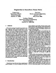
deviator of a tensor is parallel to the tensor itself. Therefore, their respective eigenvector elds are identical. Furthermore, the locations of the respective degenerate points are also identical. This, in turn, means that the topology of a tensor eld is identical to the topology of its deviator. In previous work [2], the authors presented a method for locating isolated degenerate points. However, degenerate points of double degeneracy may appear along lines or surfaces. In this paper the concept of a \control function" of a deviator is proposed. This function determines the existence of degenerate points and assists in de ning the lines and surfaces along which the degenerate points lie. Following the study of the tensor eld in the neighborhood of degenerate points, one can display a full representation of the 3-D tensor eld. Finally, the paper presents examples where degenerate points have a very important physical interpretation such Figure 1: Trisector (� < 0) and wedge (� > 0) points. as stress free point in a 2-force Boussinesq problem and the � = ad , bc and I = index. vortex core in a rotational ow. are determined by the tensor gradients at the degenerate points [5] [1]. 3 Critical Points And Degenerate Consider the partial derivatives Points ( 11 , 22 ) ( 11 , 22 ) a = 12 b = 12 (1) 12 12 c= d= 3.1 Critical Points evaluated at the degenerate point x0 . In the vicinity of x0 , Critical points are the only points in a vector eld where the expansion of the tensor components to rst-order is as � 11, 22 � a�x + b�y tangent curves may cross each other. They are character- follows: ized according to the behavior of nearby tangent curves. A 2 (2) T12 � c�x + d�y particular set of tangent curves which end on critical points are of special interest because they de ne the skeleton which where (�x; �y) are small displacements from x0 . An imporcharacterizes the global behavior of all other tangent curves tant quantity for the characterization of degenerate points in the vector eld. is the quantity A rst order critical point can be classi ed according to � = ad , bc (3) the eigenvalues of its Jacobian matrix. [3] A positive or neg- The appeal of � arises from being invariant under rotation. ative real part of an eigenvalue indicates a repelling or atWhen � < 0, the degenerate point has three hyperbolic tracting nature, respectively . The imaginary part denotes sectors. The pattern of eigenvector elds corresponding to circulation about the point. Accordingly, the critical points the trisector point is shown in Figure 1. When � > 0,x the can be classi ed as an attracting node, a repelling node, an degenerate point has one hyperbolic sector. The local patattracting focus, a repelling focus, a center or a saddle. For tern corresponds to the wedge point represented in Figures 1. more details, the reader is referred to [3] for a comprehensive The various types of degeneracies encountered in 3-D tendiscussion regarding critical point theory. sor elds can be divided into two main types. The rst, corresponding to �1 (x0 ) = �2 (x0 ) or �2 (x0 ) = �3 (x0 ) (�1 2 3 3.2 Degenerate Points are ordered in a decreasing manner), is locally 2-D, and is referred to as \double degeneracy." For example, consider The topology of a tensor eld T(x) is the topology of a degenerate point where �1 (x0 ) = �2 (x0 ) > �3 (x0 ). The its eigenvector elds v (x) [4]. Similar to critical points, tensor eld is degenerate in the plane orthogonal to v3 (x0 ) degenerate points are the basic constituents underlying the within which locally two-dimensional patterns such as wedge topology of tensor elds. Degeneracy occurs at points where points and trisectors can occur. The second type of 3-D deat least two eigenvalues are equal to each other. generacies, corresponding to �1 (x0 ) = �2 (x0 ) = �3 (x0 ), is In the case of two-dimensional tensor elds, there are only a 3-D degeneracy, and is referred to as \triple degeneracy." two eigenvalues �1 and �2 , and x0 is a degenerate point i� In this case the degeneracy is global and the structure of �1 (x0 ) = �2 (x0 ). the eigenvector trajectories in the vicinity of the degenerate Similar to critical points in vector elds, tensor elds point is fully three dimensional. The general structure of have di�erent types of degenerate points that correspond to the eigenvectors in the vicinity of a point of triple degendi�erent patterns in their neighborhoods. These patterns eracy is based upon the fundamental 2-D degeneracies in S1
δ < 0 IT = −1/2
Trisector point
S2
S1
S3
S2
S1 = S2
Wedge points
δ > 0 I = 1/2 T
@ T
T
@x
@T
@x
T
@ T
@T
T
@y
@y
T
; ;
i
planes de ned by the 3-D tensor and its expansion in the neighborhood of (x0 ) [2].
4 De nitions This section contains de nitions of basic terms that are used in the paper. The following section includes explanations. De nition 1 (Singular Point) A singular point in a tensor eld is a point where all eigenvalues of a tensor vanish, in mathematical representation, it is a zero matrix. De nition 2 (Deviator) A tensor is a deviator D i� it is trace free, T race (D) = 0, De nition 3 (Isotropic Tensor) A tensor is isotropic i� U = �� , where � is a stretch factor. ij
ij
5 Decomposition Of A Tensor Field A tensor eld in the real physical world is often very complex, therefore reducing it into a simpler form becomes very appealing. In this paper, the tensor is decomposed into a \deviator" and an \isotropic tensor" at each point in the tensor eld. Any given tensor T, can be decomposed into1 :
!
= +
T11 (x; y; z ) T12 (x; y; z ) T13 (x; y; z ) T21 (x; y; z ) T22 (x; y; z ) T23 (x; y; z ) T31 (x; y; z ) T32 (x; y; z ) T33 (x; y; z ) D11 (x; y; z ) D12 (x; y; z ) D13 (x; y; z ) D21 (x; y; z ) D22 (x; y; z ) D23 (x; y; z ) D31 (x; y; z ) D32 (x; y; z ) D33 (x; y; z ) U11 (x; y; z ) 0 0 0 U22 (x; y; z ) 0 0 0 U33 (x; y; z )
� U0
!
�
j
jj
jj
j
6 Physical Meaning Of A Deviator And An Isotropic Tensor 6.1
!
0
0 0 0 0 0 1 0 U220 . where U11 = U22 = 2 (T11 + T22 ) = � and 0 + D22 0 = 0. Clearly, D0 is the deviator of T0 . It is also D11 called a local 2-D deviator to the original tensor T. A local 2-D deviator is important when analyzing points of double degeneracy. Theorem 1 A general tensor and its deviator have the same set of eigenvectors. Proof. Let T be a symmetric tensor, it can be decomposed into a deviator D and an isotropic tensor U (see equation 4). Let � be an eigenvalue P of D, ~e be the corresponding eigenvector, and let � = 13 3=1 T be an eigenvalue of U, then D~e = �~e and since U has three identical eigenvalues U~e = �~e. Adding these two equations results in the following: T~e = (D + U) ~e = (� + � ) ~e (5) Therefore, ~e is also an eigenvector of T, i.e., T and D have the same set of eigenvectors. This is aPgeneral proof. For a 2-D tensor eld, the eigenvalue � = 12 2=1 T and the rest of the proof is the same. 11
Isotropic Tensor
Based on the previous section, one can see that the tensor U . Therefore, at any given location in the eld, it behaves the same in every (4) direction, in other words, it is an isotropic tensor. Since it is isotropic throughout the whole eld, it is of no particular physical interests to the following study.
U is an identity tensor multiplied by
where D11 + D22 + D33 = 0 and U11 = PU22 = U33 at any point in the eld. Here D = T , 13 3=1 T and U = P3 T . We denote the deviator by D and the isotropic 1 3 =1 tensor by U. A tensor can also have a \local 2-D deviator". Any given tensor can be transformed into a space in which at least one axis and one eigenvector are along the same direction, and we denote this eigenvector by e~3 . In the plane perpendicular to e~3 , the !tensor is locally 2-D. It takes the form: 0 T12 0 0 T11 0 T22 0 0 T12 0 0 �3 The locally tensor �can be decomposed into a devi� D2-D 0 D12 0 0 11 ator D = D0 D0 and an isotropic tensor U 0 =
6.2
ii
Deviator
The deviator, in contrast to the isotropic tensor, has a di�erent behavior in all 3 principal directions except at a singular point where all of its components are zero. It is indeed the deviator that represents the deviations from the originally isotropic eld and makes the entire tensor eld so complex and diverse. It is then reasonable to think of a real tensor eld as a deviator superimposed onto an isotropic tensor. By subtracting the contribution of the isotropic tensor from the tensor eld, the deviator becomes dominant and it enables us to clearly show the topology and the uctuations of the eld without the disturbance of the sometimes dominant isotropic contribution. One can think of this as a way to reduce the e�ect of the constant background, while making the variations from constancy more 12 22 pronounced. The major focus is then on the deviator, as 1 the analysis and examples in the rest of the paper are all for all the following sections are dedicated to the analysis of the 3-D space, but the theory holds for 2-D space as well topology of the deviator. ii
j
jj
ii
j
jj
ii
7 Control Functions Of The Singular 8 The Nature Of A Degenerate Point Points
Theorem 2 A tensor is of triple degeneracy i� its de-
The 3-D tensors we are considering here have the math- viator is singular. ematical form of a matrix, and one can nd the eigenvalues Proof. If a tensor T is of triple degeneracy, then T of such a tensor by investigating its characteristic equation. and its isotropic tensor U are identical. Therefore, its In the case of the deviator:
� , D ,D ,D
11
12 13
,D �,D ,D
12
where: a
D b = D
11 12
13
11
23
,D ,D �,D
= �
3
23 33
+ a�2 + b� + c (6)
= D11 + D22 + D33
D + D D c= D D
D12 D22
D13 D33
11 13
11 12 13
D12 D22 D23
(7)
D + D D D D
22 23
13
D23 D33
(8) (9)
23 33
deviator D = T , U = 0, or D is singular; On the other hand, if D is singular, then T = D + U = T.
Theorem 3 A tensor is of double degeneracy i� its de-
viator is nonsingular and one of its local 2-D deviators is singular. Proof. If a tensor T is of double degeneracy, let its eigenvalues be � and �3 , then it has one distinct eigen direction e~3 associated with �3 . We rotate the coordinate system so that one axis is along e~3 . In the transverse plane, the tensor T' is locally 2-D and degenerate, therefore, it is identical to its isotropical tensor U' and its deviator D'(also a local 2-D deviator of T) is singular. However, if the deviator D of T is singular then from Theorem 2, T has to be of triple degeneracy. Since T is only of double degeneracy, D must be nonsingular. On the other hand, if one of its local 2-D deviators D' is singular, then the local 2-D tensor T0 = U0 and T is degenerate. Since the deviator D is nonsingular, from Theorem 2, T is not of triple degeneracy. Therefore, T must be of double degeneracy. Singular points are the basic constituents of both vector elds and deviators. A singular deviator can be related to a vector with three zero components. It is natural to see the resemblance between them in topology. Since a tensor and it's deviator have the same set of eigenvectors and their degenerate points occur at the same place, they share the same topological structure. This is why the topological structure of a rst-order tensor(vector) and a second-order tensor eld have such a striking similarity. In fact, although a second-order eld is more complex than a rst-order eld, because the eigenvector elds of a second-order tensor eld has sign indeterminacy, it usually has an even simpler structure.
One can see that the coe�cients a; b and c are all tensor invariants. By de nition, D11 +D22 +D33 = 0, and therefore, a = 0. The coe�cient b can be also presented as: 1 ,D2 + D2 + D2 + 2D2 + 2D2 + 2D2 � b=, 12 13 23 2 11 22 33 (10) The characteristic equation now becomes: �3 + b� + c = 0. The standard form for the roots of this cubic equation is: q p q p �1 = 3 , 2 + � + 3 , 2 , � q q p p �2 = ! 3 , 2 + � + !2 3 , 2 , � q q p p �3 = ! 3 , 2 , � + !2 3 , 2 + � p ,� ,� Where � = 2 2 + 3 3 and ! = ,1+2 3 3 This equation has three distinct real roots when � < 0 and multiple real roots when � = 0. This study deals with symmetric tensors, and therefore the eigenvalues are always real. This, in turn, means that for all regular points in the tensor eld � has to be less than 0. The quantity � is 0 only at a degenerate point, where the characteristic equation gives multiple roots. 9 Representation Of Singularities In , � , � 2 For double roots, 2 = , 3 3 6= 0, it is a double Deviators degenerate point. For triple roots, b = c = 0, it is a triple degenerate The existence and location of degenerate points in point. a tensor eld is determined by the Control Function. From above, we see that � (x; y; z ) controls the de- Analysis of the Control Function behavior in the neighgeneracy of a deviator. We call it a \Control Function". borhood of a degenerate point also contains information c
c
c
c
c
c
c
b
c
i
p
By computing the trace and decomposing the tensor regarding the distribution of singular points in a tensor eld especially in the case that singular points appear into its deviator and the isotropic tensor: along a continuous line or surface. 0 x+y, 5 , 1 x,y 0 The control function � (x; y; z ) has maxima at a de6 3 D= @ x,y ,(x + y) + 76 , 3 0 A generate point x~0, 1 0 0 , 3 + 23 � � (x~0) = 0 (16) (11) and �( 0 ) = 0 0 1 (z + 1) 1 0 0 In the vicinity of this point, the control function can be 3 1 (z + 1) U=@ 0 0 A (17) expressed as: 3 1 (z + 1) 0 0 3 3 X @ � (x~0) � (~x) = � (x~0) + (x , x0 ) One can nd the coe�cients b and c(Equation 9and =1 @x Equation 10) of the characteristic equation, !2 3 X � 1 �2 � 1 �2 2 � 1 �2 + 2!1 (x , x 0) @x@ � (x~0) + � (12) �� b = ,4 x , =1 2 , 4 y , 2 , 3 z , 2 (18) If a singular point is located on a continuous line or " � �2 � �2 � �2# surface of singular points then the condition: � (~x) = 0 2 is satis ed along the line or on the surface respectively. c = , 2 x , 1 + 2 y , 1 , 1 z , 1 3 2 2 9 2 Substituting Equation 11 into Equation 12, results in � � the following: 1 (19) z, ! 2 2 3 X (x , x 0) @x@ � (x~0) � (~x) = 2!1 And then nd the degenerate points as follows: =1 !3 3 1. Triple Degeneracy(triple roots): b = c = 0 X 1 @ , � (x , x 0) @x � (x~0) + � � � + 3! Result: an isolated point: (x; y; z ) = 21 ; 12 ; 12 . =1 = 0 (13) 2. Double Degeneracy(double roots): , 2 �2 = ,� , 3 3 6= 0 In Equation: 13, the control function � (~x) is expanded to the nth order so that at least one of its Results: nth partial derivatives at x~0 is nonzero [6] [7]. Rear� a line: x = 12 , y = 12 ranging the function according to the order of variable ,x , 1 �2 + ,x , 1 �2 = ,z , 1 �2 (x , x0)(here ~x , x~0 is written as x , x0 , y , y0 and � a surface: 2 2 2 z , z ), results in an implicit equation in 3-D space: z
z
z
d
x ~
d~ x
i
i
i
i
i
i
i
i
i
i
i
i
i
i
i
i
c
p
0
( , x0 ) + f ,1 1 0(x , x0) ,1 (y , y0 ) + f ,1 0 1(x , x0) ,1(z , z0 ) + � � � + f0 0(y , y0) + f0 0 (z , z0 ) (14) Depending on the values of the coe�cients f 's, this equation is a representation of an object in 3-D space; Surfaces, lines and isolated points are all possibilities [6]. The following is an example of an analytical tensor: 0 =
n
fn;0;0 x n
n
n
; ;
n
; ;
n
;n;
n
; ;n
The following section contains examples of application using the methods discussed in this paper applied to problems of scienti c interest. We use both texture mapping and hyperstreamlines for display. A hyperstreamline is a trajectory that traces along the longitudinal eigenvector eld while stretching in the transverse plane under the combined action of the two transverse eigenvectors. We refer to hyperstreamlines as \major", \medium" or \minor" depending on the longitudinal eigenvector eld that de nes its trajectory [8] [9]. The rst two example refer to the deformation ten(15) sor. In the case of incompressible ow the deformation
i;j;k
0 x+y , 1 1 x,y 0 2 T = @ x , y ,(x + y) + 23 0 A 0
0
z
10 Applications
Figure 2: Major eigenvector eld of a ow past a Figure 3: Minor eigenvector eld of a ow past a wingtip. wingtip. tensor, de ned as Def = + , has a zero isotropic part and therefore is equal to its deviator. For compressible ow, the deformation tensor is composed of a deviator superimposed on a non-zero isotropic tensor which represents the rate of expansion. Therefore, a deviator describes the topological structure for both incompressible and compressible ows. For a rotational ow, inside the vortex core, ow is pure rotational. Assume that the ow advances in the z-direction and rotates around the z-axis while the velocity within the vortex core area is (,!y; !x; 0)(where ! is the angular velocity) and its deformation tensor Def (r < R) becomes singular; outside the vortex core, the velocity is ,2 (,y; x;00) and its deformation ten1 xy ,x2 + y2 0 sor Def (r > R) is: 2,2 @ ,x2 + y2 ,xy 0 A. 0 0 0 Here r is the distance from a point to the center of the vortex core and R is the radius of the vortex core. It is virtually a 2-D tensor with major and minor eigenvalues having equal magnitude but opposite sign and the medium eigenvalue remains zero. The deformation tensor is discontinuous at r = R. The angles of separatrices are calculated by using the tensor in the neighborhood of the vortex core Def (r > R) [1], it turns out that there is no real solution for the angles. This indicates that the major and minor eigenvector elds are a pair of loci in the transverse plane while medium eigenvector follows the direction of the vortex core. Studies of the alignment between vorticity and eigenvectors of the strain-rate (deformation) tensor in numerical solutions of Navier-Stokes turbulence have shown that the two principal strains with the largest absolute values (major and minor eigenvectors) lie in the equatorial plane, r
r
@ ui
@ uj
@ xj
@ xi
and the vorticity is automatically aligned to the intermediate eigenvector.2 Figure 2 and Figure 3 show the texture of a ow past a wingtip for a major eigenvector eld and a minor eigenvector eld respectively. These two eigenvectors remain in the transverse plane perpendicular to the vortex core. Images are taken from a slice of the transverse plane along the vortex core, and the two eigenvector elds form two loci as we might expect. Color encodes the magnitude of their associated eigenvalues. Figure 4 shows hyperstreamlines of the deformation tensor of a ow past a hemisphere-cylinder at a skew angle of incidence. There are two vortex cores in this ow. Two hyperstreamlines along the body are the medium eigenvectors and also de ne the direction of the vortex core. The upper ring is a minor hyperstreamline and the ring in the lower part which encloses the body is the major hyperstreamline. Pressure in a stress tensor usually comes from outside forces acting on the medium and it can be disturbingly large compared to the friction related to the viscous
ow. This makes it di�cult to see the actual e�ect from the ow itself. The bulk viscosity is the resistance of a compressible ow to the expansion. Both these two actions form an isotropic background through the eld. After subtracting the isotropic contribution from the stress tensor, the resultant, its deviator, truely re ects the nature of a viscous ow. In a Newtonian ow, the stress equals the scaled deformation tensor plus the pressure component, therefore, it behaves just like the deformation tensor of an incompressible ow. We can then predict the behavior of a stress tensor very easily from a deformation tensor, or vice versa. Figure 5 shows 2
for detailed information, please see [10] [11].
Figure 4: Deformation tensor in a ow past a hemi- Figure 5: stress tensor in a ow past a hemisphere cylinsphere cylinder at incidence der at incidence the stress tensor in a ow past a hemisphere cylinder. The major tubes in front propagate along the least compressive direction. Their trajectories show how forces propagate from the region in front of the cylinder to the surface of the body. The cross-section of the tubes are circular, indicating that the pressure component is dominant. However, viscous stresses close to the body induce slightly anisotropic cross-sections. Figure 6 shows the viscous-stress tensor in the same ow. As expected, removing the large, isotropic pressure contribution enhances the anisotropy of the tubes' cross-sections dramatically. Colors represent the magnitudes of eigenvalues of the longitudinal eigenvectors. Stress tensors are also prevalent in solid mechanics. Here we give an example of stress induced by two compressive forces acting on top of a semi-in nite solid. Unlike in uid mechanics, the stress in this problem is the compression and tension inside the solid due to the two outside forces. After taking out the isotropic part, the deviator turns out to have two triple degenerate points (singular points) and a continuous set of double degenerate points with one local 2-D deviator being singular(Theorem 3). Figure 7 shows the minor eigenvector eld (most compressive force). The arrows represent the two forces, the two balls indicate the location of singular points. The hyperstreamlines on the top surface are the separatrices [1] of the singular points which describe the topological structure in their vicinity. Inside the solid, the hyperstreamlines form trisectors of double degenerate points which indicate the pattern of topological structure in the vicinity of their singular local 2-D deviators. Colors of the hyperstreamlines encode the magnitudes
of minor eigenvalues. We also varied the strength of the two forces . It turns out that the stress free points move along a circle as the force ratio is varied. Video clip 1 shows the motion of a double degenerate point inside the solid with variation of the two forces; Video clip 2 shows the motion of two triple degenerate points on the top surface(Figure 7) with variation of two forces; Red balls indicates the degenerate points.
11 Summary Tensor analysis is a very important yet underdeveloped area both in visualization and physics. The sheer enormous volume of information and the multivariate nature have been the major hindrances. How to simplify the analysis and extract a small fraction of the data sets without any loss of information becomes the key issue. In this paper, we propose a decomposition to break a tensor eld into a deviator and an isotropic tensor. A deviator carries the essential information about the tensor eld, and describes the same topological structure. An isotropic tensor provides extra information like pressure in a stress eld or expansion of a compressible ow in a deformation tensor, it is uniform at every location in the eld yet can be dominant compared to the deviator. In order to understand the nature of a tensor eld, we primarily study its deviator. The degeneracy of a deviator is also its singularity, which explains the similarity between vector and second-order tensor elds. The study of a control function sheds light on the representation of singularities in
tional methods for their representation are still topics under development.
Acknowledgement
We are most indebted to Rajesh Batra from Stanford University for his critical comments and some of his visualization software. The authors are supported by NASA under contract NAG 2-911 which includes support from the NASA Ames Numerical Aerodynamics Simulation Program and the NASA Ames Fluid Dynamics Division, and also by NSF under grant ECS-9215145.
References Figure 6: viscous tensor in a ow past a hemisphere cylinder at incidence
Figure 7: Stress tensor induced by two compressive forces; minor hyperstreamlines a deviator as well as in the tensor eld itself. The singularities in a tensor eld often have very important physical meaning. For a deformation tensor, singularities only occur either at a vortex core or in a constant ow; for a stress tensor in solids, it is a stress free point. After being decomposed into a deviator and an isotropic tensor, a stress tensor in a compressible
ow with high pressure behaves similarly to a deformation tensor of an incompressible ow. We applied our methods to several physical problems and the results are very encouraging. For further research, it will be very interesting and useful to apply these results to actual physical applications such as vortex core detection. Also, classi cation of singularities in 3-D and implementation of computa-
[1] T. Delmarcelle, The Visualization of Second-Order Tensor Fields. PhD thesis, Stanford University, 1994. [2] Y. L. Yingmei Lavin and L. Hesselink, \The topology of three-dimensional symmetric tensor elds," in Late Breaking Hot Topics IEEE Visualization '96, pp. 43{ 46, CS Press, Los Alamitos, CA., 1996. [3] J. Helman and L. Hesselink, \Representation and display of vector eld topology in uid ow data sets," Computer, vol. 22, pp. 27{36, Aug. 1989. Also appears in Visualization in Scienti c Computing, G. M. Nielson & B. Shriver, eds. Companion videotape available from IEEE Computer Society Press. [4] A. I. Borisenko and I. E. Tarapov, Vector and Tensor Analysis with Applications. Dover Publications, New York, 1979. [5] T. Delmarcelle and L. Hesselink, \A uni ed framework for ow visualization," in Computer Visualization (R. Gallagher, ed.), ch. 5, CRC Press, 1994. [6] A. Goetz, Introduction to Di�erential Geometry. Addison-Wesly Publishing Company, Inc., 1970. [7] J.J.Stoker, Di�erential Geometry. John Wiley & Sons, Inc., 1970. [8] T. Delmarcelle and L. Hesselink, \Visualization of second-order tensor elds and matrix data," in Proc. IEEE Visualization '92, pp. 316{323, CS Press, Los Alamitos, CA., 1992. [9] T. Delmarcelle and L. Hesselink, \Visualizing secondorder tensor elds with hyperstreamlines," IEEE Computer Graphics and Applications, vol. 13, no. 4, pp. 25{ 33, 1993. [10] R. K. Wm.T. Ashurst, A.R. Kerstein and C. Gibson, \Alignment of vorticity and scalar gradient with strain rate in simulated navier-stokes turbulence," Physics of Fluids A, pp. 2343{2353, 1987. [11] J. Jimenez, \Kinematic alignment e�ects in turbulent
ows," Physics of Fluids, pp. 652{654, 1992.