Psychological Test and Assessment Modeling, Volume 56, 2014 (4), 382-404
Testing fit of latent trait models for responses and response times in tests Jochen Ranger1& Jörg-Tobias Kuhn2
Abstract The joint analysis of responses and response times in psychological tests with latent trait models has become popular recently. Although numerous such models have been proposed so far there are only few tests of model fit. In this manuscript a new approach to the evaluation of model fit is presented. The approach is based on the differences between the observed frequencies of positive or negative responses given during fixed time intervals and the corresponding expected frequencies implied by the model. Summing the squared differences yields a test statistic that is approximately chi-squared distributed. Different forms of the test can be implemented. Jointly considering all items allows for the evaluation of global fit whereas examining each item separately allows for the assessment of item fit. Depending on the definition of the frequencies one can test for specific forms of model misfit, e.g. wrong assumptions about the response time distribution, about the relation of responses and response times in the same item or about the relation of responses and response times from different items. The validity and power of the test is demonstrated in a simulation study. It can be shown that the test adheres to the nominal Type-I error rate and has high power.
Key words: item response model, response time model, fit test
1
Correspondence concerning this article should be addressed to: Jochen Ranger, PhD, Martin-LutherUniversität Halle-Wittenberg, Institut für Psychologie, Brandbergweg 23c, 06120 Halle (Saale), Germany; email:
[email protected] 2
University of Münster, Germany
Testing fit of latent trait models for responses and response times in tests
383
In computer administered tests one often records not only the responses, but also the times needed to give the responses. The availability of response time as a second quantity reflecting properties of the response process has stimulated research about the benefits of response time modelling in psychological assessment. This research has brought forth several latent traits models that relate both, the responses and the response times to latent characteristics of the test takers. One of the most prominent latent trait models for response and response time data in tests is the model of van der Linden (2007). In his model, the responses are modelled with a three-parameter logistic model and the response times with a log-normal factor model. The two models are combined under the assumption that responses and response times are independent when conditioning on the latent traits of the test takers. Other models relax the conditional independence assumption by relating the response times either to the given response or to the latent trait underlying the responses (Thissen, 1983, Gaviria, 2005). Dependencies between responses and response times can also be accounted for by incorporating response time into the item response model (Roskam, 1997, Verhelst, Verstralen, & Jansen, 1997, Wang & Hanson, 2005). A more thorough overview over these models can be found in Schnipke and Scrams (2002), van der Linden (2009) and Lee and Chen (2011). All the models mentioned in the overviews are variants of standard latent trait models and should be regarded as measurement models rather than as prescriptions of the response process. Recently, several new models have been proposed that claim to represent the response process of the test takers. These models are similar to process models in cognitive psychology and fuse cognitive psychology and psychometrics. Van der Maas, Molenaar, Maris, Kievit, and Boorsboom (2011) for example developed a latent trait version of the diffusion model which is applicable to data from achievement tests. Tuerlinckx and De Boeck (2005) used the diffusion model for data from a computerized self-report personality questionnaire. Race models for test data have been proposed by Rouder, Province, Morey, Gomez, and Heathcote (2014) and by Tuerlinckx and De Boeck (2005). Models for responses and response times in tests enrich psychological assessment by improving parameter estimation, providing additional information about the subjects and allowing for the detection of aberrant responding or the collusion between test takers (van der Linden, 2009). However, when applying such a model its adequacy for the data should be guaranteed as model based inference is only valid in case the model is an accurate representation of reality. This is especially important in psychological assessment where the results usually have serious consequences for the test takers. Nevertheless, despite the importance of model fit this topic often is neglected. One approach to the analysis of model fit consists in contrasting the sample quantiles of the response times with the theoretical quantiles implied by the model via Q-Q plots or P-P plots. Usually these plots are based on the conditional response time distribution, that is, the response time distribution when conditioning on the latent traits. However, this approach has several limitations. The same data is used for model calibration and model evaluation and this is even more problematic given the large amount of parameters being estimated, namely the item parameters and the latent traits of the test takers.
384
J. Ranger & J. T. Kuhn
Furthermore, such plots only assess the adequacy of the assumed response time distribution and several crucial assumptions of the model are not evaluated, like the interrelation of the responses and the response times in the same item or their relation in different items. The strongest point of criticism however is the fact that such plots only evaluate model fit on a global level of the data focusing on a single aspect of the response time distribution. Therefore, this approach might have low sensitivity for the presence of subtle or local forms of model violations. The low sensitivity of P-P plots can easily be demonstrated. Figure 1 depicts two P-P plots. In the first P-P plot on the left side of Figure 1 the responses and response times were generated for a test of 15 items and 200 fictitious test takers with a race model similar to the one proposed by Tuerlinckx and De Boeck (2005). In this model, a Weibull distributed random variate is associated with each response and the shorter of the two determines the observed response and response time. The date set was analyzed with the race model, estimating all item parameters by means of marginal maximum likelihood estimation and the latent traits via their posterior expectation. Then, the fit of the model was assessed with P-P plots in each item. The P-P plot on the left side shows one of the resulting plots. Note that all points are close to a straight line as it should be when the models used for data generation and data analysis are identical. In the second plot on the right side of Figure 1 the responses and response times were generated according to the model of van der Linden (2007), using the two-parameter logistic model for the responses and a standard factor model for the logarithmized response times. The data was however analyzed with the race model of Tuerlinckx and De Boeck (2005) as described before. Model fit was checked with P-P plots, of which one is shown on the right side. Despite the misfit of the model the P-P plot appears similar to the one on the right side where no misfit was present. An alternative to graphical checks of model fit are tests that evaluate observable implications of the assumed latent trait model. Such tests can be implemented by embedding the assumed model into a more flexible one. One can for example shift the response time distribution in positive and negative responses via an additional shift parameter and then test the necessity of this additional flexibility, either with a likelihood ratio test or a score test. Such a test has been implemented by van der Linden and Glas (2009) for the evaluation of the hierarchical response time model of van der Linden (2007). Tuerlinckx and De Boeck (2005) suggest a similar test for the evaluation of their race model. However, even though providing a useful test of model fit, the approach of testing for shifts of the response time distribution has two drawbacks. First, the evaluation of fit is based on a single aspect of the response time distribution and some forms of misfit like the dependency of response times from different items are hard to detect. And second, the approach is not generally applicable to all models as it requires that a shift parameter can be included. How this can be done in models such as the diffusion model is not obvious. Summing up, what is needed is an all-purpose approach to the evaluation of model fit, generally usable in all models for the evaluation of several aspects of the data. In this manuscript, a new approach to the assessment of model fit is proposed. This approach is based on a comparison of the observed and expected frequencies of responses
Testing fit of latent trait models for responses and response times in tests
385
Figure 1: P-P plots of the conditional response time distribution in a particular item from a test of 15 items based on 200 subjects. In the correct specification condition the data was generated and analyzed with the race model proposed by Tuerlinckx and De Boeck (2005). In the misspecification condition the data was generated with the model of van der Linden (2007) and analyzed with the race model proposed by Tuerlinckx and De Boeck (2005). Note that all points are very close to a straight line
given between fixed time limits. The approach provides a general framework from which several specific tests of model fit can be derived, amongst others a test that evaluates whether the response time distribution in positive and negative responses resembles the distribution implied by the model, a test that checks the validity of the implied response time distribution irrespective of the given responses or a test that assesses the local independence assumption over different items. All three tests can be implemented for single items in order to evaluate item fit or for the whole scale in order to evaluate global fit. The outline of the manuscript is as follows. In the first part of the manuscript, the general approach is described. Then, the different variants of the test are presented. And finally, the validity and the power of the tests are demonstrated in a simulation study.
Testing model fit Latent trait models for responses and responses times in tests usually assume that the joint distribution of these quantities is determined by two sets of parameters, by a vector of individual specific latent traits and by a vector of item specific parameters. Let latent
386
J. Ranger & J. T. Kuhn
trait vector θ n represent the relevant individual characteristics of subject n taking the test, like his/her ability or work pace. Let the vector of item parameters α g comprise the effects of the relevant item features on the response and response time distribution in item g like its difficulty or time intensity. The joint distribution of the responses and the response times in each item is then related to the two parameter sets by the latent trait model which specifies the distribution f xgn ,t gn |θn ;α g of the response xgn and the
response time t gn for all g=1,…,G items of a test and all n=1,…,N test takers. Note that
the function f xgn ,t gn |θn ;α g
is similar to the item characteristic of item response mod-
els. The joint distribution of all responses and response times from subject n in the test follows from the assumption of x , t x ,..., x , t ,..., t n n 1n Gn 1n Gn conditional independence which is typically made in latent trait models. The conditional independence assumption states that conditional on the latent traits θ n the observations from different items are independent. Observations from different test takers are regarded as independent too. One approach to the assessment of model fit consists in the evaluation whether the assumed conditional distributions f xgn ,t gn |θn ;α g hold true for the data. The commonly
used Q-Q and P-P plots for example contrast the quantiles of the marginal response time distribution f t gn |θn ;α g with the corresponding empirical quantiles in each item. This
practice however is far from optimal for reasons given above. Instead of checking the validity of the assumed conditional distribution one can assess the validity of the marginal distribution, that is, of the conditional distribution where the latent traits have been integrated out. Thereby, one avoids the need to estimate the latent traits of the individuals. Using the marginal distribution is common practice in psychometrics, where several well known tests take a similar approach. In factor analysis, one usually assesses whether the marginal covariance matrix implied by the model is compatible with the observed covariance matrix. In item response theory one can test the fit of a model by comparing the observed marginal tables up to a certain order with the marginal tables implied by the model. So one might wonder whether such an approach is possible in the present context also. The marginal distribution of the responses and response times in item g results from integrating the conditional distribution f xg ,t g |θ;α g over the distribution of the latent
traits f θ in the population of the test takers:
f xg , t g ; α g f xg , t g | θ; α g f θ dθ .
(1)
In latent trait models the distribution f θ is usually assumed to be the multivariate normal distribution with expectations of zero and variances of one. This assumption however is not necessary as the approach can easily be generalized to other distributions.
387
Testing fit of latent trait models for responses and response times in tests
Note, that in Equation 1 the subscript n denoting the specific subject has been dropped. Provided that the latent trait model is valid and the item parameters are known, the expected frequency of subjects reacting to item g with response x g during the time period defined by the two time limits cig and c jg can be determined from Equation 1 as
c jg
eg xg , cig , c jg N g xg , cig , c jg N
f xg , t g ; α g dt g ,
(2)
cig
where g xg , cig , c jg
denotes the related marginal probability and N is the sample size.
This expected frequency eg xg , cig , c jg
should not deviate systematically from the cor-
responding observed frequency in the sample provided that the model holds. This fact can be used for a test of model fit as follows. Define an ordered series of time limits determine
the
corresponding
c0 g 0, c1g ,..., c K 1 g , cKg and observed frequencies
t
the o g og 0, c0 g , c1g ,..., og 0, c K 1 g , cKg , og 1, c0 g , c1g ,..., og 1, c K 1 g , cKg for two possible responses xg 0 and xg 1 in the sample. Compute then the
corresponding
expected
frequencies t
e g eg 0, c0 g , c1g ,..., eg 0, c K 1 g , cKg , eg 1, c0 g , c1g ,..., eg 1, c K 1 g , cKg according to Equation 2, where maximum likelihood estimates are used as proxies for the unknown item parameters. With both quantities a residual vector can be defined by subtracting the observed and expected frequencies z g o g e g . The elements of the residual vector
indicate whether the observed distribution of the response times in positive and negative responses resembles the marginal distribution implied by the latent trait model. The residual vector can be used in order to define the test statistic
Tg ztg z g ,
(3)
where the last element of z g has been removed as z tg 1 0 . The distribution of the residuals and of the proposed test statistic will be derived in the following section.
Asymptotic distribution of the residuals and the test statistic In order to derive the distribution of the residuals and the test statistic it is assumed that the latent trait model has been calibrated with marginal maximum likelihood estimation and that the same data set is used for model calibration and model evaluation. In a first t
step, the joint distribution of the parameter estimates αˆ αˆ 1t ,..., αˆ Gt for the G test items
388
J. Ranger & J. T. Kuhn
and the observed frequencies o g in item g is determined. This result allows the specification of the joint distribution of e g and o g . Having determined the joint distribution of
e g and o g , the asymptotic distribution of the test statistic Tg can be approximated. With the conditional independence assumption the marginal distribution f x, t; α of the responses x x1,..., xG and the response times t t1,..., tG in the test follows from t
t
the conditional distributions f xg ,t g |θ;α g as G
f x,t;α f xg ,t g |θ; α g f θ dθ , g 1
(4)
where α α1t ,..., αGt are the item parameters. The score function s x, t is defined as t
the first derivative of log f x, t; α with respect to the item parameters α at their respective values, that is
s(x, t )
log f x, t; α . α
(5)
The maximum likelihood estimates αˆ are determined by the score function and can approximately be written as (Sorensen & Gianola, 2002, p.152) 1
1 N 2 1 N αˆ α log f xn ,t n ;α t N n 1 αα N
N
n 1
s xn , t n ,
(6)
where summation is over the N test takers. By the central limit theorem, the sum of the score functions, that is the last vector in Equation 6, and the observed frequencies o g are approximately distributed according to a multivariate normal distribution; see Sorensen and Gianola (2002), Agresti (2002) and Chernoff and Lehmann (1954) for more details. Define Σso g as the variance covariance matrix of the score function and the observed frequencies. The upper part of Σso g is proportional to the information matrix of the item parameters while the lower part is the variance covariance matrix of the multinomial distribution with parameters π g xg , cig , c jg of Equation 2. The covariances between the
N
elements of the score vector
s xn , tn n 1
and the vector o g are more difficult to calcu-
late. Although in theory, these covariances could be given in closed form for some latent trait models, it is much easier and faster to approximate them by a Monte Carlo method. Therefore, one has to simulate a large data set, determine the score function and the observed frequencies o g for each observation and calculate the resulting covariance
Testing fit of latent trait models for responses and response times in tests
389
matrix. Note that these calculations are not computationally expensive as only one data set has to be analyzed. Given matrix Σso g , the asymptotic variance covariance matrix Σαo ˆ g of the parameter estimates αˆ and the observed frequencies o g can be approximated by
H 1 0 Σαo Σso g ˆ g 0 I
H 1 0 , 0 I
(7)
where H is the information matrix of the item parameters and I is the identity matrix with dimensions corresponding to the length of o g . Like the sum of the score functions and the observed frequencies, the estimated item parameters and the observed frequencies are distributed asymptotically according to a multivariate normal distribution around their true values. As the expected frequencies e g are a function of the estimated item parameters αˆ g , their distribution can be derived with the Delta method (Casella & Berger, 2002, p.245). Define the Jacobian matrix of e g as
Δ
eg . αtg
(8)
The Delta method is based on Δ and allows the determination of the joint distribution of the expected frequencies e g and the observed frequencies o g . This distribution is approximately multivariate normal, with means resembling the expected frequencies and the variance covariance matrix t
Δ 0 Δ 0 Σe g o g Σαo ˆ g . 0 I 0 I
(9)
The residuals are just the difference between the observed and expected frequencies, that is, z g o g e g . As the residuals z g are a linear combination of the multivariate normally distributed quantities e g and o g , they are also distributed according to a multivariate normal distribution with zero mean and variance covariance matrix given by t
Σz g I I Σe g o g I I .
(10)
Due to the joint normality of the residuals z g , the asymptotic distribution of the test statistic Tg , which was defined in Equation 3 as the sum of the squared residuals except the last one, is a mixture of 2 random variates (Yuan & Bentler, 2010). An approximation of this distribution can be derived as follows: Let 1,..., d be the nonzero eigenvalues of the part of Σ z g that has been used for the calculation of Tg , that is, matrix Σ z g
390
J. Ranger & J. T. Kuhn
d i and b i i 1 i 1 i 1 distribution of the test statistic Tg can be approximated by d
d
without the last row and column. With a i2
2
d
i2 , the i 1
Tg ~ a b2 .
(11)
This approximation is of wide use in categorical data analysis and structural equation modeling and dates back to Welch (1938); for a thorough overview over the development and the performance of this approximation see Yuan and Bentler (2010).
Alternative versions of the test In the preceding section only the residuals in a single item were considered. However, the approach is more general as it might appear on first sight. In fact, all one needs are observed and expected frequencies. Different definitions of these quantities induce different tests of model fit. Two modifications are possible. The first modification refers to the definition of the observed and expected frequencies in the single items. One can ignore the type of response and simply determine the number of responses given during fixed time intervals. The quantities og xg , cig , c jg and
eg xg , cig , c jg
simplify to og cig , c jg
and eg cig , c jg
in this case. As the number of
categories is limited – the expected frequencies eg cig , c jg
should be greater than five
as it is typically recommended for -statistics – this focus on response time allows for a finer resolution of the time axis. Therefore, this version of the test has sometimes more power to detect violations concerning the marginal response time distribution. Small deviations in the tail of the response time distribution might be more easily detected for example. 2
Instead of using responses and response times in a single item one can also define categories with the responses and response times from item pairs. Let the two time limits cig and c jg constitute a time interval for item g and the two time limits ckh and clh a time
interval for item h. The quantity ogh xg , xh , cig , c jg , ckh , clh
denotes the frequency of
individuals responding with response x g to item g during interval cig , c jg and with response xh to item h during interval ckh , clh . This quantity can be compared to
egh xg , xh , cig , c jg , ckh , clh , the corresponding expected frequency. Large deviations be-
tween observed and expected frequencies indicate a violation of the conditional independence assumption. Such violations occur in item bundles for example. Both alternative definitions of expected and observed frequencies constitute test statistics similar to
Testing fit of latent trait models for responses and response times in tests
391
the one proposed in Equation 3. The derivation of their asymptotic distribution is straightforward, one only has to adapt Equation 8 slightly. The second modification refers to the number of items considered at the same time. Instead of examining each item separately, one can test the similarity of the observed and expected frequencies in all items jointly. This makes a test of global fit which has higher power than item specific tests in case small model violations in all items sum up. Again, the necessary adaptations are straightforward. The test statistic T zt z is now based on the residuals z z1,..., zG in all items. In order to derive the asymptotic distribution the proceeding remains largely the same. One only has to modify the Jacobian matrix given in Equation 8, which now contains the derivatives with respect to all item parameters.
Simulation study In order to demonstrate the usefulness of the tests, five simulation studies were conducted. These studies differed in the way the model used for data analysis was misspecified. In the first simulation study there was no model misspecification such that this study served in order to explore the Type-I error rate of the tests. The second simulation study explored whether the tests can detect that the model used for data generation and the model used for data analysis are completely different. The third simulation study assessed whether the test is sensitive to a misspecification of the joint distribution of the responses and response times in the same item. The fourth simulation study dealt with the power of the test to detect violations of the local independence assumption in responses and response times from different items. And in the fifth simulation study it was investigated whether the test reveals the presence of rapid guessing. All simulation studies were based on a test of 15 binary scored items. Simulation samples of 250, 500 and 1000 subjects were considered. The variance of the response times was systematically varied by creating a scenario with rather low variance and a scenario with high variance. Therefore, in each simulation study 3×2 simulation conditions were distinguished. For each simulation condition, 500 simulation samples were generated. The simulation study was implemented in the statistical software environment R (R Development Core Team, 2009). All scripts can be obtained from the authors on request.
Simulation study 1 In the first simulation study the models used for data generation and data analysis were identical, both times being the race model proposed by Tuerlinckx and De Boeck (2005). The race model assumes that in each item the positive and negative response compete and that the response is uttered that can be generated faster. This model was chosen as a representative of a nonstandard latent trait model, for which the best approach to fit testing is not obvious. The data was generated according to the model as follows. First, a latent trait value was drawn from the standard normal distribution for every fictitious test taker. This latent
392
J. Ranger & J. T. Kuhn
trait determined the scale parameters of two Weibull distributions, one associated with the positive response and the other one associated with the negative response. The shape parameters of the two Weibull distributions were identical, not depending on the latent trait. Then, two response times were drawn from the two Weibull distributions. In the model these two quantities are regarded as the latent time requirement needed for generating the positive and negative response. Of these two latent response times the smaller of the two was registered. This quantity was considered as the observed response time and the associated response as the given response. According to this proceeding, altogether 15 responses and response times were generated for each subject, mimicking the subject’s data in a test of 15 items. When generating the response times care was taken that the simulated data sets resembled real data sets. In a first simulation condition the item parameters were chosen such that the first two moments of the generated response times were similar to the data from a visual array comparison task intended for the assessment of working memory capacity. With these item parameters the solution probabilities in the items ranged approximately from 0.25 to 0.75, the average response times from 1.75s to 2.75s and the variance from 1.00 to 2.00. However, often there is a lot of noise in response time data and therefore the variance of the response times was increased in a second simulation condition. This was achieved with a second set of item parameters. With these alternative parameter values, the solution probabilities ranged from 0.25 to 0.75, the average response times from 2.5s to 5.0s and the variances from 5.00 to 16.00. With the second condition we wanted to assess the test’s performance in case of a more unfavourable signal to noise ratio or rather in case the systematic variance due to the latent trait is small in comparison to the unexplained variance of the response times. For each simulation condition data sets with 250, 500 and 1000 subjects were fabricated. This generated a 2×3 simulation design. More information about the simulation study (e.g. the item parameters of the 15 items) can be obtained from the authors. Having generated the data, the item parameters were estimated with marginal maximum likelihood estimation. The likelihood function was based on the correct model, such that in the first simulation study the models used for data generation and data analysis were the same. The maximum likelihood estimator converged in all samples and the item parameter recovery was good. Having calibrated the model six different tests of model fit were calculated. The first test was the test of item fit that was described in detail in the previous section. This test relies on the frequencies of positive and negative responses given during fixed time intervals in each item. For the test the time axis was divided into 9 segments at 8 more or less equally spaced time limits ranging from 0.7 to 3.1 in the first item. The time limits in the remaining items were similar. The time limits were chosen in order to guarantee a sufficient number of expected responses in each time interval and to cover the range of the response times as uniformly as possible. Then, the observed and expected frequencies for the altogether 9 response time × 2 response categories were determined. The fit test was calculated item wise as described above. The expected information matrix needed in Equation 7 was approximated by a Monte Carlo method via the observed
Testing fit of latent trait models for responses and response times in tests
393
information matrix in 10000 new observations, which were generated with the assumed model and the estimated item parameters. Two alternative tests of item fit were implemented as well. The first alternative test was based on the response times solely and compared the observed and expected frequencies of responses given between fixed time limits irrespective of the response. For this test the time axis was divided into a grid defined by 13 time limits ranging from 0.5 to 3.3 in the first item. The time limits used in the remaining items were similar. This alternative test was supposed to be more sensitive to misspecification of the response time distribution than the standard test of item fit described before. The second alternative test was based on data from item pairs. Therefore, 14 item pairs were formed by pairing subsequent items. In the first item pair, the response times in the constituent items were categorized at the two time limits 1.3 and 2.2. This generated two discrete response times with three levels each. Then, the resulting two discrete response times were cross tabulated with the two binary responses. This defined altogether 2×2×3×3 categories, for which the observed and expected frequencies were compared with the test described above. In the other item pairs the proceeding was identical except for the location of the time limits. In samples of 250 subjects, the time axis was only divided at one time limit as the expected frequencies would have been too small otherwise. This second alternative test was supposed to detect violations of the local independence assumption across items with higher power. Each of the three item specific tests was supplemented by its corresponding test of global fit. Thereby, the deviations of expected and observed frequencies were compared in all items simultaneously. In total, three tests of item fit were calculated for each of the 15 items and three tests of global fit for each simulation sample. The empirical rejection rates of the different tests can be found in Figure 2 for different nominal Type-I error rates. Note that the results concerning the item specific versions of the tests have been averaged over the items. As there was no model misfit to be detected the empirical rejection rates should resemble the nominal Type-I error rates closely. In addition to the empirical rejection rates of the tests Figure 2 contains two dotted lines. Points outside the region defined by the dotted lines indicate significant deviations from the nominal Type-I error rate on α=0.05. But note that strictly speaking the rejection region is only valid for the rejection rates of the global fit tests and not for the averaged rejection rates reported for the tests of item fit. As can be seen in Figure 2, the tests of item fit closely adhere to the nominal Type-I error rate in all sample sizes and the two parameter sets. The performance of the global tests of model fit is not as good. Although in samples of 1000 subjects the rejection rates are close to the nominal Type-I error rate there are slight deviations from the nominal Type-I error rate in samples of 500 and 250 subjects. This might be due to the fact that the tests of global fit are based on the residuals of all items and require a precise estimation of the residuals’ covariance matrix, which is too imprecise in small samples. But even in the most disadvantageous case the difference between the empirical rejection rate and the nominal Type-I error rate is small and might be beyond practical significance.
394
J. Ranger & J. T. Kuhn
Figure 2: Empirical rejection rate of six tests for different nominal Type-I error rates α and six simulation conditions defined by three sample sizes N and two variance-mean relations in the first simulation study without misspecification. The tests are denoted as follows: TX–I/TX–G: Item specific and global test based on responses and response times, T–I/T–G: Item specific and global test based on responses times, TT–I/TT–G: Item specific and global test based on data from item pairs. Points outside the dotted lines deviate significantly from the nominal Type-I error rate
Simulation study 2 Adherence to the nominal Type-I error rate is a necessary requirement for a test, but does not guarantee that the test is useful. Therefore, the power of the test was explored in subsequent simulation studies. In the second simulation study it was investigated whether the tests are able to distinguish measurement orientated response time models from cognitive-psychometric models empirically. This is a question of theoretical relevance. Often, it is difficult to distinguish one latent trait model from the other in case the two models make similar predictions; see Figure 1 for an example. In the second simulation study the responses and response times were generated according to the model of van der Linden (2007), which follows a more traditional approach to data analysis. The model is composed of two
Testing fit of latent trait models for responses and response times in tests
395
separate submodels, a three-parameter logistic model for the responses and a standard factor model for the logarithmized response times. One distinct latent trait is assumed to underlie each of the two submodels. The submodels are combined on a higher level by assuming correlated latent traits. Although the data sets were generated with the model of van der Linden (2007), they were analyzed with the race model as described before. Here, the race model figures as a representative of cognitive process models. Note that when using the race model the misspecification is limited to the response time distribution, which is a log-normal distribution in the model of van der Linden (2007) and a Weibull distribution in the race model of Tuerlinckx and De Boeck (2005). The marginal distribution of the responses is not misspecified as in both models the distribution comes down to a two-parameter logistic model in case there in no guessing. Data sets were generated for a test of 15 items and 250, 500 or 1000 subjects depending on the simulation condition. Again, two item parameter sets were used in order to vary
Figure 3: Empirical rejection rate of six tests for different nominal Type-I error rates α and six simulation conditions defined by three sample sizes N and two variance-mean relations in the second simulation study where the data was generated according to the model of van der Linden (2007) and analyzed with the model of Tuerlinckx and De Boeck (2005). The tests are denoted as follows: TX–I/TX–G: Item specific and global test based on responses and response times, T–I/T–G: Item specific and global test based on responses times, TT–I/TT–G: Item specific and global test based on data from item pairs. Note that the plots show the power of the tests
396
J. Ranger & J. T. Kuhn
the signal to noise ratio or rather the communalities when slightly abusing the terminology of factor analysis. The specific values of the item parameters were chosen such that the generated response times had first two moments similar to the response times in the first simulation study. The guessing parameter of the three-parameter logistic model was set to zero. Having generated the data according to the model of van der Linden (2007), the race model of Tuerlinckx and De Boeck (2005) was used for data analysis. Item parameters were estimated via marginal maximum likelihood estimation and the six tests of model fit were calculated. The time limits used for categorizing the response times were slightly adapted to the different range of the response time distribution in the second simulation study, but their number as well as the general principle for their placement remained the same. The empirical rejection rates of the tests can be found in Figure 3. Note that the results concerning the item specific versions of the tests have been averaged over the items. Irrespective of the amount of variance the tests based on response time have the highest power. This illustrates that tailoring the test to the nature of misfit improves the detection of model violations. When compared to the tests of item fit the test of global fit is superior. This is due to the fact that misfit was present in all items and accumulates in the test statistic. With misfit limited to single items the picture might have been different. Nevertheless, it might be wise to test for global model misfit first and then proceed with item specific tests.
Simulation study 3 In the third simulation study the misspecification concerned the relationship between the responses and response times in the same item. Namely, it was investigated whether the test can detect an additional shift of negative responses. There is some controversy in response time modelling whether incorrect response times are the result of a wrong solution process or the result of a motivational process that terminates the futile efforts of an individual. In the second case, the response times in wrong responses should be significantly longer than the response times in correct responses. A test for this violation of the conditional independence assumption was proposed by van der Linden and Glas (2009) for the hierarchical model of van der Linden (2007). Whether the actual framework can be used for this research question also was investigated in the third simulation study. For a start the data was generated as in the first simulation study by using the race model with exactly the same item parameters. Then, model misfit was created by adding the fixed amount of 0.25s to the response times in positive responses. Given the mean and standard deviation of the marginal response time distribution this shift of the response times in positive responses could not be detected by a visual inspection of the response time distribution. Six simulation conditions were defined by crossing three sample sizes with two variance conditions. The data sets were analyzed with the race model and marginal maximum likelihood estimation as before, ignoring the shift of positive response times. Even though the model used for data analysis was not adequate for the data set, the recovery of the item parameters was rather good. This is further evidence that the amount of model misfit was rather modest. Having estimated the item parameters, the six
Testing fit of latent trait models for responses and response times in tests
397
tests of model fit were calculated as described before. The location of the time limits was slightly adapted to the greater spread of the response times. The empirical rejection rates of the test can be found in Figure 4. The rejection rates of the item specific tests have been averaged over the items. As can be seen in Figure 4, the two tests based on the response time distribution can not detect the misfit of the model. The performance of the two tests based on item pairs is better, but not good in the condition with high variance. The two tests based on the responses and response times in the same item are superior to their direct competitors in both conditions. But only the global version has high power in the low and the high variance condition. These findings illustrate two points. First, some forms of model misfit do not emerge in the response time distribution. It is the association of the responses and response times in the same item that contains the information about the model inadequacy. And second, it might be better to consider all items jointly than to check each item separately for model violations.
Figure 4: Empirical rejection rate of six tests for different nominal Type-I error rates α and six simulation conditions defined by three sample sizes N and two variance-mean relations in the third simulation study where the response times in positive responses were shifted by a fixed amount. The tests are denoted as follows: TX–I/TX–G: Item specific and global test based on responses and response times, T–I/T–G: Item specific and global test based on responses times, TT–I/TT–G: Item specific and global test based on data from item pairs. Note that the plots show the power of the tests.
398
J. Ranger & J. T. Kuhn
Simulation study 4 In the fourth simulation study the local independence assumption concerning responses and response times from different items was violated. This occurs sometimes in very similar items that are based on the same content or are logically dependent. However, when investigating violations of the local independence assumption one has to take care that the misfit is limited to the association of the responses and response times from different items and nothing else. This can be accomplished by copulas that allow for dependencies between random variates but leave their marginal distributions unchanged. For the fourth simulation study a copula was combined with the race model as follows. As in the first simulation study, responses and response times were generated by a race of two latent Weibull distributed response times. However, in order to create violations of the local independence assumption six items were chosen and assorted to three item pairs. The pairs were formed by items (1,2), items (6,7) and items (11,12). In each of these item pairs the latent response times were related by a normal copula. The latent response times from different items had a coefficient of correlation of 0.25 in the normal copula. No extra association was created between the two latent response times in the same item. The item parameters of the race model were identical to the values used in the first simulation study. Having generated 500 data sets for each simulation condition (two parameter sets and three sample sizes) they were analyzed with the race model without accounting for the extra association in the item pairs. Despite using a misspecified model for data analyses, the parameters were virtually unbiased. Again, the six tests of model fit were calculated as described before. The empirical rejection rates of the test can be found in Figure 5, split into results for items / item pairs without model fit (item 1,2,6,7,11,12 and the pairs mentioned above) and items / item pairs with model fit (the remaining items and item pairs). The results for the global tests are presented with the results for misfitting items. Figure 5 illustrates two findings. Tests that are based on the data from single items are not capable of detecting extra association between data from different items. This can be seen from the lower part of Figure 5 where the four tests based on the responses and response times in the same item have a rejection rate near the applied α value. This is hardly surprising as single items were conform to the race model. The tests based on item pairs have considerable power in case of large samples. Compared to the item specific test the global test performs somewhat worse. This is not unreasonable as only 3 of the 14 item pairs considered by the global test were affected by local dependencies. Note that the item specific version of the test has a very low rate of false alarms. As is apparent in the upper part of Figure 5 the rejection rate of the test is around the applied level of α in the item pairs that are not affected by local dependencies.
Testing fit of latent trait models for responses and response times in tests
399
Figure 5: Empirical rejection rate of six tests for different nominal Type-I error rates α and six simulation conditions defined by three sample sizes N and two variance-mean relations in the fourth simulation study where the local independence assumption was violated in three item pairs. The tests are denoted as follows: TX–I/TX–G: Item specific and global test based on responses and response times, T–I/T–G: Item specific and global test based on responses times, TT–I/TT–G: Item specific and global test based on data from item pairs. Results are given for items with misfit and items without misfit.
Simulation study 5 In the fifths simulation study it was investigated whether the tests can detect rapid guessing. Rapid guessing is a problem in low stakes testing and occurs in case unmotivated test takers do not try to solve the items seriously but simply guess in order to finish the test rapidly. Rapid guessing was simulated as follows. In a first step, the data was gener-
400
J. Ranger & J. T. Kuhn
ated as before with the race model and the item parameters of the first simulation study. Having generated the data 10% of the subjects were chosen randomly and assigned to the group of rapid guessers. Their responses were replaced by random draws from a binomial distribution with success probability of 0.2. This was supposed to be a realistic solution probability for a multiple choice test with five response options. The response times were drawn from a Weibull distribution with shape and location parameter of 1. The resulting response times had an expectation of 1 and a variance of 1. Quickness and low variance is a typical characteristic of rapid guesses. However, even though a subgroup of respondents answered significantly faster the resulting distribution was not bimodal such that the presence of two groups was not apparent. The data sets were analysed with the race model as before. Then, the tests of model fit were calculated. The time limits used for the tests were slightly adapted to the different distribution of the response times. The empirical rejection rates of the test can be found in Figure 6. The rejection rates of the item specific tests have been averaged over the items.
Figure 6: Empirical rejection rate of six tests for different nominal Type-I error rates α and six simulation conditions defined by three sample sizes N and two variance-mean relations in the fifth simulation study where rapid guessers were present. The tests are denoted as follows: TX–I/TX–G: Item specific and global test based on responses and response times, T–I/T–G: Item specific and global test based on responses times, TT–I/TT–G: Item specific and global test based on data from item pairs. Note that the plots show the power of the tests
Testing fit of latent trait models for responses and response times in tests
401
Figure 6 suggests that none of the item specific versions of the tests can detect the presence of rapid guessers with high probability. This is not really surprising as rapid guessing is a phenomenon that affects the whole test and not single items. The global tests are more powerful. The most powerful test is the test based on the responses and response times from item pairs. Rapid guessing probably increases the marginal association between the responses and response times and this is detected by the test. However, with samples of 500 subjects and more the differences between the global tests are of no practical importance anymore.
Discussion Latent trait models for the joint distribution of the responses and response times in psychological tests have become popular. These models have a high level of practical use, as they allow for the identification of aberrant responses (van der Linden & van KrimpenStoop, 2003), increase the precision of item parameter and trait estimates (van der Linden, Klein Entink, & Fox, 2010, Ferrando & Lorenzo-Seva, 2007), permit the consideration of response time for item selection in adaptive testing (van der Linden, 2008) and provide a measure of the respondent’s speed as a second quantity, which can be used for psychological assessment (Stricker & Alderton, 1999, Genser, 1988). Some of these models are even based on stringent assumptions about the response process and provide a better understanding of the latent traits, which are measured by the latent trait model (van der Maas et al., 2011, Tuerlinckx & De Boeck, 2005, Vandekerckhove, Tuerlinckx, & Lee, 2011). However, model based interpretation and model based inference requires that the model used for data analysis is valid and is able to represent the structure of the data well, as otherwise conclusions might be wrong. This is especially important in educational testing where test results often have serious consequences for test takers. Although much work has been dedicated to the development of new latent trait models, less effort has been invested in the development of tests for model fit. In this manuscript, a general framework for tests of model fit was presented. The proposed approach is rather flexible and allows for different implementations of specific tests. As the simulation study revealed the tests adhere to the nominal Type-I error rate closely even under unfavourable conditions of small samples and large residual variance. The power of the tests however differs for the different implementations of the test. None of the tests can detect all forms of misspecification. Distinguishing a cognitive process model from a more standard latent trait model for responses and response times is a relatively easy task and all implementations of the tests are helpful here. This demonstrates that it is possible to distinguish process models from standard measurement models empirically, a question of theoretical importance for cognitive psychometrics. Other model violations are harder to detect and no test has high power in all forms of model violations. This is shown quite plainly by the fifth simulation study, where only the tests based on the item pairs perform well. Therefore, in order to detect specific forms of misfit with high power one needs a tests which explicitly focuses on this specific aspect of the distributions. This suggests that a thorough analysis of model fit must not limit itself to just one aspect of the distribution. The simulation study also demonstrates that
402
J. Ranger & J. T. Kuhn
global tests are often superior to an item specific analysis of model fit in case small deviations in single items accumulate. Consequently, the general practice of using graphical checks of model fit might not be enough. Several other fit tests for response and response time models exist. Van der Linden and Glas (2009) proposed several score tests for the assessment of the hierarchical response time model of van der Linden (2007). These tests can be used for more or less the same purpose as the tests proposed in this manuscript. However, the score tests are intimately connected with the hierarchical model and the log-normal distribution. Generalizations to different models are not straightforward. In contrast, the proposed approach is a flexible framework that can be used for models of all kinds irrespective of a specific response time distribution. In addition to the score function (which one usually needs for maximum likelihood estimation already) not much additional calculations are necessary. Contrary to the score tests, the actual test requires arbitrary decisions concerning the number and location of the cut points. These decisions can have a substantial influence on the power of the test. As an example, consider the fifth simulation study with rapid guessing. The power of the global test based on response time and equally spaced quantiles was 0.41 for α=0.05 in samples of 250 subjects. Moving the time limits towards zero and dividing the lower range of the time axis into a finer grid increases the power to 0.46. Moving the time limits towards the response time maxima and concentrating on large response times had virtually no effect on the detection rate. More important was the number of cut points. By varying the number of the cut points the power could be increased up to 0.60. In fact, this dependency of the power on the way the expected frequencies are defined is the motive for the different versions of the test, which detect different forms of misfit. Insofar the dependency of the results on the way the data is categorized is not necessarily a weakness. Recently, several models for response and response time data in psychological tests have been proposed. However, in order to use these models in psychological assessment sound tests of model and item fit are necessary. Tests of item fit are useful for test development when a subset of valid items has to be selected from a large item pool. Global tests are needed in order to validate the measurement model used for the final test. This is of utter most importance as the application of a measurement model has to be justified in case its application has consequences for the test taker or third parties. Therefore, the proposed tests of model fit hopefully support psychometricians in developing valid measurement models for responses and response times in tests.
References Agresti, A. (2002). Categorical data analysis. New York: Wiley. Casella, G., & Berger, R. (2002). Statistical inference. Pacific Grove: Duxbury. Chernoff, H., & Lehmann, E. (1954). The use of maximum likelihood estimates in 2 tests for goodness of fit. The Annals of Mathematical Statistics, 25, 579–586.
Testing fit of latent trait models for responses and response times in tests
403
Ferrando, P., & Lorenzo-Seva, U. (2007). An item response theory model for incorporating response time data in binary personality items. Applied Psychological Measurement, 31, 525–543. Gaviria, J. (2005). Increase in precision when estimating parameters in computer assisted testing using response times. Quality & Quantity, 39, 45–69. Genser, S. (1988). Computer response time measurement of mood, fatigue and symptom scale items: Implications for scale response time uses. Computers in Human Behavior, 4, 95– 109. Lee, Y., & Chen, H. (2011). A review of recent response-time analyses in educational testing. Psychological Test and Assessment Modeling, 53, 359–379. R Development Core Team. (2009). R: A language and environment for statistical computing [Computer software manual]. Vienna, Austria. Retrieved from http://www.R-project.org (ISBN 3-900051-07-0) Roskam, E. (1997). Models for speed and time-limit tests. In W. van der Linden & R. Hambelton (Eds.), Handbook of modern item response theory (pp. 187–208). New York: Springer. Rouder, J., Province, J., Morey, R., Gomez, P., & Heathcote, A. (2014). The lognormal race: A cognitive-process model of choice and latency with desirable psychometric properties. Psychometrika, Online First. Schnipke, D., & Scrams, D. (2002). Exploring issues of examinee behavior: Insights gained from response-time analyses. In C. Mills, M. Potenza, J. Fremer, & W. Ward (Eds.), Computer-based testing: Building the foundation for future assessments (pp. 237–266). Mahwah: Lawrence Erlbaum. Sorensen, D., & Gianola, D. (2002). Likelihood, Bayesian, and MCMC methods in quantitative genetics. Berlin: Springer. Stricker, L., & Alderton, D. (1999). Using response latency measures for a biographical inventory. Military Psychology, 11, 169–188. Thissen, D. (1983). Timed testing: An approach using item response theory. In D. Weiss (Ed.), New horizons in testing: Latent trait test theory and computerized adaptive testing (pp. 179–203). New York: Academic Press. Tuerlinckx, F., & De Boeck, P. (2005). Two interpretations of the discrimination parameter. Psychometrika, 70, 629–650. van der Linden, W. (2007). A hierarchical framework for modeling speed and accuracy on test items. Psychometrika, 72, 287–308. van der Linden, W. (2008). Using response times for item selection in adaptive tests. Journal of Educational and Behavioral Statistics, 31, 5–20. van der Linden, W. (2009). Conceptual issues in response-time modeling. Journal of Educational Measurement, 46, 247–272. van der Linden, W., & Glas, C. (2009). Statistical tests of conditional independence between responses and/or response times on test items. Psychometrika, 75, 120–139.
404
J. Ranger & J. T. Kuhn
van der Linden, W., & Klein Entink, R., & Fox, J. (2010). IRT parameter estimation with response times as collateral information. Applied Psychological Measurement, 34, 327– 347. van der Linden, W., & van Krimpen-Stoop, E. (2003). Using response times to detect aberrant responses in computerized adaptive testing. Psychometrika, 68, 251-265. van der Maas, H., Molenaar, D., Maris, G., Kievit, R., & Boorsboom, D. (2011). Cognitive psychology meets psychometric theory: On the relation between process models for decision making and latent variable models for individual differences. Psychological Review, 118, 339–356. Vandekerckhove, J., & Tuerlinckx, F., & Lee, M. (2011). Hierarchical diffusion models for two-choice response times. Psychological Methods, 16, 44–62. Verhelst, N., Verstralen, H., & Jansen, M. (1997). A logistic model for time-limit tests. In W. van der Linden & R. Hambelton (Eds.), Handbook of modern item response theory (pp. 169–185). New York: Springer. Wang, T., & Hanson, B. (2005). Development and calibration of an item response model that incorporates response time. Applied Psychological Measurement, 29, 323–339. Welch, B. (1938). The significance of the difference between two means when the population variances are unequal. Biometrika, 29, 350–362. Yuan, K., & Bentler, P. (2010). Two simple approximations to the distributions of quadratic forms. British Journal of Mathematical and Statistical Psychology, 63, 273–291.