Testing local versions of correlation coefficients - GISc in Greece

Testing local versions of correlation coefficients Stamatis KALOGIROU Lecturer, Department of Geography, Harokopio University of Athens, El. Venizelou 70, Kallithea – 17676, Athens, Greece, Email: [email protected] Abstract The aim of this paper is to define and test local versions of standard correlation coefficients in statistical analysis. This research is motivated by the increasing number of applications using local versions of explanatory spatial data analysis methods such as local regression. One example of the latter is the Geographically Weighted Regression that allows for the researcher to check for the existence of spatial non-stationarity in the relationships between a geographic phenomenon and its determinants. In this paper, a local version of Pearson correlation coefficient is defined and applied to internal migration data. The results suggest that globally independent variables are not necessarily independent locally, thus the independence criterion may be violated when local regression analysis is performed. The work presented here is work-in-progress and will evolve along with the development of statistical software necessary for testing local versions of statistical tests. Keywords: Statistical Inference in Geography, Spatial Analysis, Correlation, Geographically Weighted Regression. 1. Introduction and Background An increasing number of applications of local regression methods in physical and human geography appear in the recent literature along with the development of specialised software such as GeoDa (Anselin, 2003a; 2003b; 2004), GWR 3.0 (Fotheringham et al., 2002a) and various packages in R such as spdep and spgwr (Bivand, 2010). These methodologies are trying to address the theoretically expected variable response to a stimulus across space when spatial data are concerned. More specifically, local regression methods such as the Geographically Weighted Regression (GWR) claim to account for local relationships that may be hidden or missed when a global regression is applied. However, the statistical inference in local regression methods is still an open field for basic research with recent

contributions by Brunsdon (2009 and Wheeler and Paez (2010). The contribution of this paper is to define and test local versions of standard correlation coefficients in statistical analysis and more specifically to test a local version of Pearson Correlation Coefficient for the pairs of the explanatory variables of a regression model. The latter is simpler approach for checking multicollinearity among explanatory variables in local regression compared to the local diagnostics tools such as the VIF presented by Wheeler (Wheeler, 2006; 2007). Motivation for this work has been the lack of of-the-self local multicollinearity diagnostics in local regression methods that has been recognised by Wheeler and Tiefelsdorf (2005) as well as by Wheeler and Paez (2010). For example, the GWR analysis recently included as a tool in ESRI’s ArcGIS 9.3.x is meant to check for local multicollinearity in the independent variables. However, in case of a significant multicollinearity the software returns an error code/message suggesting the problem but it does not inform of the variables locally correlated. Thus the user has to guess and word on a trial-and-error basis that is a rather user unfriendly approach and discourages the check of statistical inference that is key to knowledge discovery in spatial data and processes. One way to identify local multicollinearity is by developing the relevant local diagnostics. The latter would allow the researcher to identify those pairs of variables that are independent globally but highly correlated locally. In line with the latter, this paper introduces a simple approach to check for local multicollinearity among a set of explanatory variables. This is the calculation of the Pearson Correlation Coefficient for each pair of variables based on a fixed number of nearest neighbours as well as the corresponding t-student test statistic. One could refer to this as a local Pearson Correlation Coefficient. This statistic allows for a postregression analysis of statistical inference and is more relevant to regression techniques such as the GWR with an adaptive kernel. It is necessary to note that correlation coefficients for the identification of correlation of local parameter estimates resulted in by the application of GWR have been already calculated (Wheeler and Tiefelsdorf, 2005) but they should not be confused with the analysis presented here that refers to the explanatory variables and not their local parameter estimates. The proposed statistic is tested in a simple model of internal outmigration for Sweden. The latter refers to gross internal migration recorded for Swedish municipalities in 2008.

The following section presents the methodology for calculating local Pearson correlation coefficients, the Geographically Weighted Regression and the data this analysis has been applied to. The results of the data analysis as well as some concluding remarks follow. It is necessary to note that this is work-in-progress thus any comments and suggestions to the author will be more than welcome. 2. Data and Methodology The data source for both migration and the two explanatory variables is Statistics Sweden (SCB, 2010). Any person that moves address is recorded as a migrant in the Swedish registry data. Aggregate data are published annually as the last census was in 1991. Out-migration rates used here is the ratio of internal out-migration in a year divided by the mean population in the same year, multiplied by 1000. The selected age group of males aged 35 – 44 reflects male adults racing children and who’s internal migration behaviour can be usually explained by key socioeconomic variables (Kalogirou, 2003; 2010). The geographical level of analysis here is the municipality. There are 290 municipalities in Sweden. Two variables have been selected here as potential determinants of internal out-migration rates based on previous findings for their statistical significant effect (Kalogirou, 2010) .These variable are: a. the proportion of males aged 35-44 with high education attainment, and b. the proportion of males aged 35 – 44 who are divorced. In the former variable high education attainment is considered the completion of post-secondary education 3 years or more (ISCED97 level 5A) or post-graduate education (ISCED97 level 6) according to the Swedish Education System (SCB, 2010) that adopted the International Standard Classification of Education (ISCED 97). 3.1 Local Pearson Correlation The Pearson Correlation Coefficient is a standard statistic for checking collinearity in the independent variable for linear regression models that are calibrated using Ordinary Least Squares (OLS). The formula to calculate this coefficient r in order to check for the correlation between two variables X and Y that have a normal distribution, mean values of x and y , and standard deviations of sx and sy , respectively, is:

 xi  x  y i   s x  s y i1  n

r

 

n 1

y   

n

 xi  x ( yi  y) i 1

( n  1) sx s y

n

 x  x ( y  y) i



i

i 1 n

( n  1)

n

 x  x    y  y  2

i

i 1

(n 1)

(1)

2

i

i 1

( n  1)

where n is the number of observations. The equation can also be written as follows: n

r

 x  x ( y i

i

 y)

i1

n

n

  x  x   y 2

i

i 1

 y

(2)

2

i

i 1

The Pearson correlation coefficient r is statistically significant at a given significant level a if the absolute value of t given by Equation 3 is higher than the value of the two tailed t-student distribution for n-2 degrees of freedom and a significance level.

t

r 1  r2 n2

t 

r n2 1 r 2

(3)

where n is the number of observations. The local version of the above two statistics is calculated as follows. The software developed for this purpose reads a dataset which includes the values of the explanatory variables for each observation, the x and y coordinates of the location each observation refers to and a number of nearest neighbours k set by the user. Based on an Euclidean distance matrix automatically calculated for all pairs of observations, the algorithm identifies the k nearest neighbours for the location of each observation (inclusive of the observation on the location) in order to created a local subset and calculates a Pearson correlation coefficient (Equation 2) for each pair of explanatory variables based on this subset. It also calculates the corresponding t test statistics (Equation 3). The results are saved on a text file at a form of local correlation coefficient and t test statistics matrices.

The number of nearest neighbours is determined by the application of GWR analysis using an adaptive kernel. 3.2 Internal migration modelling In the last four decades there have been several exploratory and explanatory studies of migration (see for example Champion, 1989; Stillwell et al., 1995; Atkins et al., 1996; Rogers et al., 2002). Most of the literature on migration modelling has been focused on destination choice models (Lowry, 1966; Congdon, 1989; Fik and Mulligan, 1990; Pellegrini and Fotheringham, 1999; Boyle and Flowerdew, 1993) where the gravity model has typically been applied. In this paper, the first stage of an internal migration process is being modelled; this is the decision to move out of an area to another area within a country. This concerns the definition of a model of out-migration rates per thousand people over a set of explanatory factors. The methodology applied here adopts Kalogirou’s (2003; 2006; and 2010) work on local models of internal migration using the Geographically Weighted Regression (GWR) method (Fotheringham et al., 2000; 2002a). The main contribution of internal migration models for Sweden in recent years is the work of Thomas Niedomysl (2004; 2005; 2006; 2007; and 2008) whose publication is a good reference for evaluating the results of this work. In this paper, a simple internal out-migration model is defined based on the conclusions of previous research that found divorce rates and high levels of education attainment to play an important role on the decision of men in Sweden to migrate internally in Sweden (Kalogirou, 2010). The model has been calibrated using Ordinary Least Squares and GWR. GWR allows for the examination of the existence of spatial non-stationarity in the relationship between outmigration rates and the two explanatory variables of the above model. A post-regression analysis involves the check for the potential existence of significant multicollinearity among the two variables due to a small and changing subset of observations in the local models. 4. Migration modelling results and statistical inference In advance of fitting a migration model it is necessary to study the distribution and spatial structure of the dependent variable. Internal out-migration rates for males aged 35-44 for Swedish municipalities in 2008 range from 16.11 to 131.02 per thousand people in this age

group. The examination for the existence of spatial autocorrelation in this data through the calculation of the Moran’s I (Anselin, 2004) suggests a positive spatial autocorrelation. The Moran’s I is 0.3322. Furthermore by calculating local versions of Moran’s I it is possible to identify spatial clusters of municipalities with similarly high or low out-migration rates as expected due to positive spatial autocorrelation. Figure 1 shows a map of out-migration rates as well as the centres of spatial clusters with high rates in the areas of Stockholm, Malmö/Lund and Filipstad/Hällefors. There are also several clusters of low out-migration rates in rural areas across Sweden.

Figure 1. Map of out-migration rates and spatial clusters centres The existence of spatial autocorrelation in the dependent variable violates the independence criterion of linear regression and it is thus necessary to calibrate local models of internal outmigration. Since this is just to test for local multicollinearity in the globally independent explanatory variables, only a global and a local linear out-migration model is fit. For the global model the ordinary least squares methods is applied whereas for the local model the

Geographically Weighted Regression model is applied. The results of the data calibration are presented in Table 1. Both explanatory variables have a positive effect on out-migration that is significant at the 99.9% confidence lever. The coefficient of determination (R2) is rather low (0.146) which is expected since there are many variables that affect the decision to migrate (Kalogirou, 2003). However, in the local model the effect of both variables ranges from a negative effect to a positive effect. The Monte Carlo test (Hope, 1968) provides empirical evidence for a significant spatial variation in the local parameter estimates of both high education attainment and divorce rates for males aged 35 -44. Based on both R2 (0.506) and AIC, the local model has a better performance than the global model. The latter is also confirmed by lower and spatially independent model residuals in the case of GWR compared to the OLS (Figure 4). Table 1. Global and local regression results OLS Variable

Parameter

Sig.

Estimates

GWR Parameter

Monte

Estimates

Carlo test

Constant

9.914

0.038

-61.621 - 75.398

0.000

High Educated

0.405

0.000

-2.069 - 1.472

0.000

Proportion Divorced

3.392

0.000

-2.660 - 9.749

0.010

R2

0.146

0.506

Adjusted R2

0.137

0.405

2359.650

2314.672

290

41

AIC Observations /Nearest Neighbours

Figure 2. Local parameter estimates of the proportion of men aged 35 – 44 with a high level of education attainment The local parameter estimates as well as the local t test values of the proportion of men aged 35 – 44 with a high level of education attainment are shown in Figure 2. A strong and significantly positive effect is apparent in the area of Stockholm and Uppsala Län and a strong and significantly negative effect in the areas within and around Örebro and Kalmar Län.

Figure 3. Local parameter estimates of the proportion men aged 35 – 44 who are divorced The local parameter estimates as well as the local t test values of the proportion of men aged 35 – 44 who are divorced are shown in Figure 3. A strong and significantly positive effect is apparent in municipalities in three areas; Stockholm and Uppsala Län; Skåne, Kronobergs and Hallands Län; and Västra Götalands län. A negative but not statistically significant effect appears in the areas in North Sweden and in central South Sweden as seen in Figure 3. Based on the above mentioned effect there is an apparent urban-rural divide. There is a positive effect of both variables on internal out-migration in urban areas and a negative effect in rural areas in North Sweden and those areas in the South that are between the three main metropolitan areas of Stockholm, Göteborg and Malmö.

Figure 4. OLS and GWR model residuals

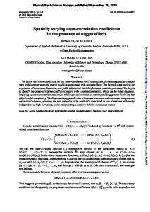
The local parameter estimates of both explanatory variables are indeed correlated. The Pearson correlation coefficient is 0.649 and statistically significant in the 99.9% confidence level confirming Wheeler’s and Tiefelsdorf’s (2005) criticism about the potential weakness of the application of GWR. However, here we are interested in the correlation of the values of the explanatory variables locally. For this purpose local Pearson correlation coefficients and the corresponding t-test values have been computed and presented in Figure 5. The global Pearson correlation coefficient between the two explanatory variables is -0.061 and the corresponding t value is -1,035. Thus, it can be argued that there is apparently no correlation between the two variables and the independence criterion for the OLS is satisfied. However, Local Pearson correlation coefficients calculated for the location of each observation assuming 41 nearest neighbours (those of the GWR) range from -0.423 to 0.263 as shown in Figure 5. Out of 290 local Pearson correlation coefficients 16 found to be significant at the 95% confidence level for 40 degrees of freedom. The threshold of t student

test in order to reject the null hypothesis (that the correlation coefficient is 0) in the latter case is T = 2.021.

Figure 5. Local Pearson Correlation Coefficients and the corresponding t-test values

5. Concluding remarks In this paper global and local versions of standard correlation coefficients have been calculated in order to check for multicollinearity in the explanatory variables in global and local regression models, respectively. A simple internal out-migration model for males aged 35-44 in Sweden in 2008 has been defined and fit. The global model (OLS) resulted in an apparent significant positive effect on the decision to migrate of both the proportion of males aged 35-44 with high education attainment and the proportion of males aged 35 – 44 who are divorced. When the data were calibrated locally by using the Geographically Weighted Regression method, a significantly varying effect of both explanatory variables was apparent.

There latter was strongly and significantly positive in urban areas and insignificantly negative in rural areas. The local Pearson correlation coefficients for the two explanatory variables presented in this paper provide some evidence for the existence of significant local correlation in the values of these variables in some local models, even though these variables are globally independent. Thus, the independence criterion may be satisfied in global linear regression but violated when local linear regression analysis is performed. Therefore, it is necessary for the researcher to always perform analysis of statistical inference in order to provide adequate evidence for the significance of the empirical findings of GWR analysis. The work and findings presented here obviously need further investigation. More diagnostic tools should be developed and check in a more complex statistical models with several explanatory variables.

6. References Anselin, L. (2003a) An Introduction to EDA with GeoDa, Spatial Analysis Laboratory (SAL), Department of Agricultural and Consumer Economics, University of Illinois, UrbanaChampaign, IL. Anselin, L. (2003b) GeoDa 0.9 User’s Guide, Spatial Analysis Laboratory (SAL). Department of Agricultural and Consumer Economics, University of Illinois, Urbana-Champaign, IL. Anselin, L. (2004) GeoDa 0.95i Release Notes, Spatial Analysis Laboratory (SAL), Department of Agricultural and Consumer Economics, University of Illinois, UrbanaChampaign, IL. Atkins, D., Champion, T., Coombes, M., Dorling, D., and Woodward, R. (1996) Urban Trends in England: Latest Evidence from the 1991 Census, London: HMSO. Bivand, R.S. (2010) Spatial Econometric Functions in R, in Handbook of Applied Spatial Analysis (Ed.) M. M. Fischer and A. Getis, Berlin: Springer-Verlag: 53 – 71.

Boyle, P.J., and Flowerdew, R (1993) Modelling sparse interaction matrices: interward migration in Hereford and Worcester, and the underdispersion problem, Environment and Planning A, 25: 1201 – 1209. Brunsdon, C. (2009) Statistical Inference for Geographical Processes, in The SAGE handbook of spatial analysis (Ed) A.S. Fotheringham and P. Rogerson, London: Sage Publications: 207 – 224. Champion, A.G. (1989) Counterurbanization: The Changing Pace and Nature of Population Deconcentration, London: Edward Arnold. Congdon, P. (1989) Modelling migration flows between areas: an analysis for London using the Census and OPCS longitudinal study, Regional Studies, 23: 87 – 103. Fik, T. J., and Mulligan, G. F. (1990) Spatial Flows and competing central places: towards general theory of hierarchical interaction, Environment and planning A, 22: 527 – 549. Fotheringham, A.S., Brunsdon, C., Charlton, M.E (2000) Quantitative Geography, London: Sage Publications. Fotheringham, A.S., Brunsdon, C., Charlton, M. (2002a) Geographically Weighted Regression: the analysis of spatially varying relationships, Chichester: John Wiley and Sons. Fotheringham, A.S., Barmby, T., Brunsdon, C., Champion, T., Charlton, M., Kalogirou, S., Tremayne, A., Rees, P., Eyre, H., Macgill, J., Stillwell, J., Bramley, G., Hollis, J. (2002b) Development of a Migration Model: Analytical and Practical Enhancements, London: Office of the Deputy Prime Minister. Hope, A.C.A. (1968) A simplified Monte Carlo significance test procedure, Journal of the Royal Statistical Society, Series B (methodological), 30 (3): 582–598. Kalogirou, S., (2003) The Statistical Analysis And Modelling Of Internal Migration Flows Within England And Wales, PhD Thesis, School of Geography, Politics and Sociology, University of Newcastle upon Tyne, UK.

Kalogirou, S., Putting Sweden on the map of internal migration modelling, British Society for Population Studies 2006 Conference, The University of Southampton, Southampton, UK, 1820 September 2006. Kalogirou, S. (2010) The application of contemporary spatial analysis methods in internal migration: the case of Sweden, Geographies, Greece (in press). (in Greek) Lowry, I. S., (1966) Migration and metropolitan growth: two analytical models, Sun Francisco: Chandler. Niedomysl, T. (2004) Evaluating the effects of place marketing campaigns on interregional migration in Sweden, Environment and Planning A, 36 (11): 1991–2009. Niedomysl, T. (2005) Tourism and interregional migration in Sweden: an explorative approach, Population, Space and Place, 11(3): 187–204. Niedomysl, T. (2006) Migration and Place Attractiveness, Geografiska Regionstudier Nr 68, Uppsala Universitet (Published Ph.D. thesis). Niedomysl, T. (2007) Promoting rural municipalities to attract new residents: an evaluation of the effects, Geoforum, 38(4): 698–709. Niedomysl, T. (2008) Residential preferences for interregional migration in Sweden: demographic, socio-economic and geographical determinants, Environment and Planning A, 40(5): 1109–1131. Pellegrini, P.A., and Fotheringham, A.S. (2002) Modelling special choice: a review and synthesis of in a migration context, Progress in Human Geography, 26: 487 – 510. Rogers, A., Raymer, J., and Willekens, F. (2002) Capturing the age and spatial structures of migration, Environment and Planning A, 34: 341 – 359. SCB (2010) Statistiska Centralbyrån, http://www.scb.se, last visited on 10 June 2010.

Stillwell, J., Duke-Williams, O., and Rees, P. (1995) Time series migration in Britain: the context for 1991 Census analysis, Papers in Regional Science, 74 (4): 341 – 359. Wheeler, D. C. (2006) Diagnostic tools and remedial methods for collinearity in linear regression models with spatially varying coefficients, PhD Thesis, Ohio State University, Department of Geography. Wheeler, D.C. (2007) Diagnostic tools and a remedial method for collinearity in geographically weighted regression, Environment and Planning A, 39(10):2464-2481 Wheeler, D., Tiefelsdorf, M. (2005) Multicollinearity and correlation among local regression coefficients in geographically weighted regression, Journal of Geographical Systems, 7:161– 187. Wheeler, D.C., Paez, A. (2010) Geographically Weighted Regression, in Handbook of Applied Spatial Analysis (Ed) M. M. Fischer and A. Getis, Berlin: Springer-Verlag: 461-486.