Tests for error correlation in the functional linear model

Tests for error correlation in the functional linear model Robertas Gabrys Utah State University

Lajos Horváth University of Utah

Piotr Kokoszka Utah State University

Abstract The paper proposes two inferential tests for error correlation in the functional linear model, which complement the available graphical goodness of fit checks. To construct them, finite dimensional residuals are computed in two different ways, and then their autocorrelations are suitably defined. From these autocorrelation matrices, two quadratic forms are constructed whose limiting distribution are chi–squared with known numbers of degrees of freedom (different for the two forms). The asymptotic approximations are suitable for moderate sample sizes. The test statistics can be relatively easily computed using the R package fda, or similar MATLAB software. Application of the tests is illustrated on magnetometer and financial data. The asymptotic theory emphasizes the differences between the standard vector linear regression and the functional linear regression. To understand the behavior of the residuals obtained from the functional linear model, the interplay of three types of approximation errors must be considered, whose sources are: projection on a finite dimensional subspace, estimation of the optimal subspace, estimation of the regression kernel.

1

Introduction

The last decade has seen the emergence of the functional data analysis (FDA) as a useful area of statistics which provides convenient and informative tools for the analysis of data objects of large dimension. The influential book of Ramsay and Silverman (2005) provides compelling examples of the usefulness of this approach. Functional data arise in many contexts. This paper is motivated by our work with data obtained from very precise measurements at fine temporal grids which arise in engineering, physical sciences and finance. At the other end of the spectrum are sparse data measured with error which are transformed into curves via procedures that involve smoothing. Such data arise, for example, in longitudinal studies on human subjects or in biology, and wherever frequent, 1

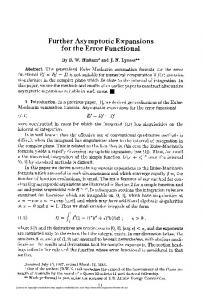
precise measurements are not feasible. Our methodology and theory are applicable to such data after they have been appropriately transformed into functional curves. Many such procedures are now available. Like its classical counterpart, the functional linear model stands out as a particularly useful tool, and has consequently been thoroughly studied and extensively applied, see Cuevas et al. (2002), Malfait and Ramsay (2003), Cardot et al. (2003), Chiou et al. (2004), M¨ uller and Stadtm¨ uller (2005), Yao, M¨ uller and Wang (2005a, 2005b) Cai and Hall (2006), Chiou and M¨ uller (2007), Li and Hsing (2007), Reiss and Ogden (2007, 2009a 2009b), among many others. For any statistical model, it is important to evaluate its suitability for particular data. In the context of the multivariate linear regression, well established approaches exist, but for the functional linear model, only the paper of Chiou and M¨ uller (2007) addresses the diagnostics in any depth. These authors emphasize the role of the functional residuals εî (t) = Yî (t) − Yi (t), where the Yi (t) are the response curves, and the Yî (t) are the fitted curves, and propose a number of graphical tools, akin to the usual residual plots, which offer a fast and convenient way of assessing the goodness of fit. They also propose a test statistic based on Cook’s distance, Cook (1977) or Cook and Weisberg (1982), whose null distribution can be computed by randomizing a binning scheme. We propose two goodness–of–fit tests aimed at detecting serial correlation in the error functions εn (t) in the fully functional model Z (1.1) Yn (t) = ψ(t, s)Xn (s)ds + εn (t), n = 1, 2, . . . , N. The assumption of iid εn underlies all inferential procedures for model (1.1) proposed to date. As in the multivariate regression, error correlation affects various variance estimates, and, consequently, confidence regions and distributions of test statistics. In particular, prediction based on LS estimation is no longer optimal. In the context of scalar data, these facts are well–known and go back at least to Cochrane and Orcutt (1949). If functional error correlation is detected, currently available inferential procedures cannot be used. At this point, no inferential procedures for the functional linear model with correlated errors are available, and it is hoped that this paper will motivate research in this direction. For scalar data, the relevant research is very extensive, so we mention only the influential papers of Sacks and Ylvisaker (1966) and Rao and Griliches (1969), and refer to textbook treatments in Chapters 9 and 10 of Seber and Lee (2003), Chapter 8 of Hamilton (1989) and Section 13.5 of Bowerman and O’Connell (1990). The general idea is that when dependence in errors is detected, it must be modeled, and inference must be suitably adjusted. The methodology of Chiou and M¨ uller (2007) was not designed to detect error correlation, and can leave it undetected. Figure 1.1 shows diagnostic plots of Chiou and M¨ uller 2

(2007) obtained for synthetic data that follow a functional linear model with highly correlated errors. These plots exhibit almost ideal football shapes. It is equally easy to construct examples in which our methodology fails to detect departures from model (1.1), but the graphs of Chiou and M¨ uller (2007) immediately show it. The simplest such ex2 ample is given by Yn (t) = Xn (t) + εn (t) with iid εn . Thus, the methods we propose are complimentary tools designed to test the validity of specification (1.1) with iid errors against the alternative of correlation in the errors. Despite a complex asymptotic theory, the null distribution of both test statistics we propose is asymptotically chi–squared, which turns out to be a good approximation in finite samples. The test statistics are relatively easy to compute, an R code is available upon request. They can be viewed as nontrivial refinements of the ideas of Durbin and Watson (1950, 1951, 1971), see also Chatfield (1998) and Section 10.4.4 of Seber and Lee (2003), who introduced tests for serial correlation in the standard linear regression. Their statistics are functions of sample autocorrelations of the residuals, but their asymptotic distributions depend on the distribution of the regressors, and so various additional steps and rough approximations are required, see Thiel and Nagar (1961) and Thiel (1965), among others. To overcome these difficulties, Schmoyer (1994) proposed permutation tests based on quadratic forms of the residuals. We appropriately define residual autocorrelations, and their quadratic forms (not the quadratic forms of the residuals as in Schmoyer (1994)), in such a way that the asymptotic distribution is the standard chi– squared distribution. The complexity of the requisite asymptotic theory is due to the fact that in order to construct a computable test statistic, finite dimensional objects reflecting the relevant properties of the infinite dimensional unobservable errors εn (t) must be constructed. In the standard regression setting, the explanatory variables live in a finite dimensional Euclidean space with a fixed (standard) basis, and the residuals reflect the effect of parameter estimation. In the functional setting, before any estimation can be undertaken, the dimension of the data must be reduced, typically by projecting on an “optimal” finite dimensional subspace. This projection operation introduces an error. Next, the “optimal subspace” must be estimated, and this introduces another error. Finally, estimation of the kernel ψ(·, ·) introduces still another error. Our asymptotic approach focuses on the impact of these errors. We do not consider the dimensions of the optimal projection spaces growing to infinity with the sample size. Such an asymptotic analysis is much more complex; in a simpler setting it was developed by Panaretos et al. (2010). The two methods proposed in this paper start with two ways of defining the residuals. Method I uses projections of all curves on the functional principal components of the regressors, and so is closer to the standard regression in that one common basis is used. This approach is also useful for testing the stability of model (1.1) against a change point alternative, see Horváth et al. (2009). Method II uses two bases: the eigenfunctions of 3

Figure 1.1 Diagnostic plots of Chiou and Müller (2007) for a synthetic data set simulated

0.2 −0.2

−0.1

0.0

0.1

0.2 0.1 0.0 −0.1 −0.2

3rd Residual FPC Score

according to model (1.1) in which the errors εn follow the functional autoregressive model of Bosq (2000).

0.0

0.5

1.0

−1.0

−0.5

0.0

0.5

1.0

−1.0

−0.5

0.0

0.5

1.0

−0.1

0.0

0.1

0.2

−0.2

−0.1

0.0

0.1

0.2

−0.2

−0.1

0.0

0.1

0.2

0.2 −1.0

−0.5

0.0

0.5

−0.4

−0.2

0.0

0.2 0.0 −0.2 −0.4 0.5 0.0 −0.5 −1.0

2nd Residual FPC Score 1st Residual FPC Score

−0.2

0.4

−0.5

0.4

−1.0

1st Fitted FPC Score

2nd Fitted FPC Score

4

the covariance operators of the regressors and of the responses. The remainder of the paper is organized as follows. Section 2 introduces the assumptions and the notation. Section 3 develops the setting for the least squares estimation needed define the residuals used in Method I. After these preliminaries, both tests are described in Section 4, with the asymptotic theory presented in Section 5. The finite sample performance is evaluated in Section 6 through a simulation study, and further examined in Section 7 by applying both methods to magnetometer and financial data. All proofs are collected in Sections 8, 9 and 10.

2

Preliminaries

We denote by L2 the space of square integrable functions on the unit interval, and by h·, ·i and || · || the usual inner product and the norm it generates. The usual conditions imposed on model (1.1) are collected in the following assumption. Assumption 2.1 The errors εn are independent identically distributed mean zero elements of L2 satisfying E||εn ||4 < ∞. The covariates Xn are independent identically distributed mean zero elements of L2 satisfying E||Xn ||4 < ∞. The sequences {Xn } and {εn } are independent. For data collected sequentially over time, the regressors Xn need not be independent. We formalize the notion of dependence in functional observations using the notion of L4 – m–approximability advocated in other contexts by Hörmann (2008), Berkes et al. (2009), Aue et al. (2009), and used for functional data by Hörmann and Kokoszka (2010) and Aue et al. (2010). We now list the assumptions we need to establish the asymptotic theory. For ease of reference, we repeat some conditions contained in Assumption 2.1; the weak dependence of the {Xn } is quantified in Conditions (A2) and (A5). Assumption 2.1 will be needed to state intermediate results. (A1) The εn are independent, identically distributed with Eεn = 0 and E||εn ||4 < ∞. (A2) Each Xn admits the representation Xn = g(αn , αn−1 , . . .), in which the αk are independent, identically distributed elements of a measurable space S, and g : S ∞ → L2 is a measurable function. (A3) The sequences {εn } and {αn } are independent. (A4) EXn = 0, E||Xn ||4 < ∞. (A5) There are c0 > 0 and κ > 2 such that ¡

E||Xn − Xn(k) ||4 5

¢1/4

≤ c0 k −κ ,

where (k)

(k)

Xn(k) = g(αn , αn−1 , . . . , αn−k+1 , αn−k , αn−k−1 , . . .), (k)

and where the α`

are independent copies of α0 .

Condition (A2) means that the sequence {Xn } admits a causal representation known as a Bernoulli shift. It follows from (A2) that {Xn } is stationary and ergodic. The structure of the function g(·) is not important, it can be a linear or a highly nonlinear function. What matters is that according to (A5), {Xn } is weakly dependent, as it can be approximated with sequences of k–dependent variables, and the approximation improves as k increases. Several examples of functional sequences satisfying (A2), (A4) and (A5) can be found in Hörmann and Kokoszka (2010) and Aue et al. (2010). They include functional linear, bilinear and conditionally heteroskedastic processes. We denote by C the covariance operator of the Xi defined by C(x) = E[hX, xi X], x ∈ 2 L , where X has the same distribution as the Xi . By λk and vk , we denote, correspondingly, the eigenvalues and the eigenfunctions of C. The corresponding objects for the Yi are denoted Γ, γk , uk , so that C(vk ) = λk vk ,

Xn =

∞ X

ξni vi , ξni = hvi , Xn i ;

i=1

Γ(uk ) = γk uk ,

Yn =

∞ X

ζnj uj , ζnj = huj , Yn i .

j=1

In practice, we must replace the population eigenfunctions and eigenvalues by their ˆ k , vˆk , γˆk , uˆk defined as the eigenelements of the empirical covariempirical counterparts λ ance operators (we assume EXn (t) = 0) ˆ C(x) = N −1

N X

hXn , xi Xn ,

x ∈ L2 ,

n=1

ˆ The empirical scores are also denoted with the ”hat”, i.e. by and analogously defined Γ. ξˆni and ζˆnj . We often refer to the vi , uj as the functional principal components (FPC’s), and to the vî , uˆj as the empirical functional principal components (EFPC’s). To state the alternative, we must impose dependence conditions on the εn . We use the same conditions that we imposed on the Xn , because then the asymptotic arguments under HA can use the results derived for the Xn under H0 . Specifically, we introduce the following assumptions: (B1) Eεn = 0 and E||εn ||4 < ∞. (B2) Each εn admits the representation εn = h(un , un−1 , . . .), 6

in which the uk are independent, identically distributed elements of a measurable space S, and h : S ∞ → L2 is a measurable function. (B3) The sequences {un } and {αn } are independent. (B4) There are c0 > 0 and κ > 2 such that ¡

4 E||εn − ε(k) n ||

¢1/4

≤ c0 k −κ ,

where (k)

(k)

ε(k) n = h(un , un−1 , . . . , un−k+1 , un−k , un−k−1 , . . .), (k)

and where the u`

are independent copies of u0 .

The tests proposed in Section 4 detect dependence which manifests itself in a correlation between εn and εn+h for at least one h. Following Bosq (2000), we say that εn and εn+h are uncorrelated if E[hεn , xi hεn+h , yi] = 0 for all x, y ∈ L2 . If {ej } is any orthonormal basis in L2 , this is equivalent to E[hεn , ei i hεn+h , ej i] = 0 for all i, j. The two methods introduced in Section 4 detect the alternatives with ei = vi (Method I) and ei = ui (Method II). These methods test for correlation up to lag H, and use the FPC vi , i ≤ p, and ui , i ≤ q. With this background, we can state the null and alternative hypotheses as follows. H0 : Model (1.1) holds together with Assumptions (A1)–(A5). The key assumption is (A1), i.e. the independence of the εn . HA,I : Model (1.1) holds together with Assumptions, (A2), (A4), (A5), (B1)–(B4), and E[hε0 , vi i hεh , vj i] 6= 0 for some 1 ≤ h ≤ H and 1 ≤ i, j ≤ p. HA,II : Model (1.1) holds together with Assumptions, (A2), (A4), (A5), (B1)–(B4), and E[hε0 , ui i hεh , uj i] 6= 0 for some 1 ≤ h ≤ H and 1 ≤ i, j ≤ q. Note that the ui are well defined under the alternative, because (A2), (A4), (A5) and (B1)–(B4) imply that the Yn form a stationary sequence. In the proofs, we will often use the following result established in Hörmann and Kokoszka (2010) and Aue et al. (2010). In Theorem 2.1, and in the following, we set cˆj = sign(hvj , vˆj i). Theorem 2.1 Suppose Assumptions (A2), (A4) and (A5) hold, and (2.1)

λ1 > λ2 > . . . > λp > λp+1 .

Then, for each 1 ≤ j ≤ p, ¤ £ (2.2) lim sup N E ||ˆ cj vˆj − vj ||2 < ∞,

i h ˆ j |2 < ∞. lim sup N E |λj − λ N →∞

N →∞

7

3

Least squares estimation

In this section we show how model (1.1) can be cast into a standard estimable form. The idea is different from the usual approaches, e.g in Ramsay and Silverman (2005) and Yao et al. (2005b), so a detailed exposition is necessary. The goal is to obtain clearly defined residuals which can be used to construct a goodness–of–fit test. This section carefully explains the three steps involved in the construction of the residuals in the setting of model (1.1). The idea is that the curves are represented by their coordinates with respect to the FPC’s of the Xn , e.g. Ynk = hYn , vk i is the projection of the nth response onto the kth largest FPC. A formal linear model for these coordinates is constructed and estimated by least squares. This formal model does not however satisfy the usual assumptions due to the effect of the projection of infinite dimensional curves on a finite dimensional subspace, and so its asymptotic analysis is delicate. Since the vk form a basis in L2 ([0, 1]), the products vi (t)vj (s) form a basis in L2 ([0, 1]× [0, 1]). Thus, if ψ(·, ·) is a Hilbert–Schmidt kernel, then (3.1)

ψ(t, s) =

∞ X

ψij vi (t)vj (s),

i,j=1

where ψij =

RR

ψ(t, s)vi (t)vj (s)dtds. Therefore, Z ψ(t, s)Xn (s)ds =

∞ X

ψij vi (t) hXn , vj i .

i,j=1

Hence, for any 1 ≤ k ≤ p, we have (3.2)

Ynk =

p X

ψkj ξnj + enk + ηnk ,

j=1

where Ynk = hYn , vk i ,

ξnj = hXn , vj i ,

and where ηnk =

∞ X

enk = hεn , vk i ,

ψkj hXn , vj i .

j=p+1

We combine the errors enk and ηnk by setting δnk = enk + ηnk . Note that the δnk are no longer iid. Setting Xn = [ξn1 , . . . , ξnp ]T

Yn = [Yn1 , . . . , Ynp ]T , 8

δ n = [δn1 , . . . , δnp ]T ,

ψ = [ψ11 , . . . , ψ1p , ψ21 , . . . , ψ2p . . . , ψp1 , . . . , ψpp ]T , we rewrite (3.2) as Yn = Zn ψ + δ n ,

n = 1, 2, . . . , N,

where each Zn is a p × p2 matrix    Zn =  

XTn 0Tp · · · 0Tp XTn · · · .. .. .. . . . T T 0p 0p · · ·

0Tp 0Tp .. .

    

XTn

with 0p = [0, . . . , 0]T . Finally, defining the N p × 1 vectors Y and δ and the N p × p2 matrix Z by       δ1 Z1 Y1  Z2   Y2   δ2        Z =  . , Y =  . , δ =  . , . . .  .   .   .  ZN δN YN we obtain the following linear model (3.3)

Y = Zψ + δ.

Note that (3.3) is not a standard linear model. Firstly, the design matrix Z is random. Secondly, Z and δ are not independent. The error term δ in (3.3) consists of two parts: the projections of the εn , and the remainder of an infinite sum. Thus, while (3.3) looks like the standard linear model, the existing asymptotic results do not apply to it, and a new asymptotic analysis involving the interplay of the various approximation errors is needed. Representation (3.3) leads to the formal “least squares estimator” for ψ is ˆ = (ZT Z)−1 ZT Y = ψ + (ZT Z)−1 ZT δ. ψ

(3.4)

which cannot be computed because the vk must be replaced by the vˆk . Now we turn to the effect of replacing the vk by the vˆk . Projecting onto the vˆk , we are “estimating” the random vector (3.5)

e = [ˆ ψ c1 ψ11 cˆ1 , . . . , cˆ1 ψ1p cˆp , . . . , cˆp ψp1 cˆ1 , . . . , cˆp ψpp cˆp ]T .

with the “estimator”

e ∧ = (Z ˆ ˆT Y ˆ −1 Z ˆ T Z) ψ

9

obtained by replacing the vk by the vˆk in (3.4). It vector of dimension p2 with the p × p matrix  ∧ ∧ ψ˜11 ψ˜12 ···  ψ˜∧ ψ˜∧ · · · 21 22 e∧ =  (3.6) Ψ  .. .. .. p  . . . ∧ ∧ ˜ ˜ ψ ψ ··· p1

p2

will be convenient to associate this ∧ ψ˜1p ∧ ψ˜2p .. . ˜ ψ∧

   . 

pp

It can be shown that if the regularity conditions of Hall and Hosseini-Nasab (2006) hold, then (3.7)

e ∧ − ψ) e = [C ˆ − ψ) + Q−1 (RN 1 + RN 2 ) + oP (1), b ⊗ C] b N 1/2 (ψ N 1/2 (ψ

where  (3.8)

  b C= 

cˆ1 0 · · · 0 cˆ2 · · · .. .. .. . . . 0 0 ···

0 0 .. .



   , 

  Q = Ip ⊗  

cˆp

λ1 0 · · · 0 λ2 · · · .. .. .. . . . 0 0 ···

0 0 .. .

   , 

λp

and where ⊗ denotes the Kronecker product of two matrices. The terms RN 1 and RN 2 are P PN −1/2 linear functionals of N −1/2 N n=1 Xn (t) and N n=1 {Xn (t)Xn (s) − E[Xn (t)Xn (s)]}. 1/2 ˆ The limits of N (ψ − ψ), RN 1 and RN 2 are thus jointly Gaussian, but the asymptotic e∧ − ψ e does not follow due to the random signs cˆj . It does however follow normality of ψ e ∧ − ψ) e = OP (1), and this relation does not require the regularfrom (3.7) that N 1/2 (ψ ity assumptions of Hall and Hosseini-Nasab (2006). The rate N 1/2 is optimal, i.e. if P e ∧ − ψ) e → aN /N 1/2 → ∞, then aN (ψ ∞. This is exactly the result that will be used in the following, and we state it here as Proposition 3.1. We need the following additional assumption. Assumption 3.1 The coefficients ψij of the kernel ψ(·, ·) satisfy

P∞ i,j=1

|ψij | < ∞.

e∧ − ψ e = OP (N −1/2 ). Proposition 3.1 If Assumptions (A1)–(A5) and 3.1 hold, then ψ The proof of Proposition 3.1 is fairly technical and is developed in Aue et al. (2010). Relation (3.7) shows that replacing the vk by the vˆk changes the asymptotic distribue ∧ is complex and cannot be used directly, this tion. While the limiting distribution of ψ estimator itself can be used to construct a feasible goodness–of–fit test.

10

4

Testing the independence of model errors

We propose two test statistics, (4.5) and (4.8), which can be used to test the assumption that the errors εn in (1.1) are iid functions in L2 . These statistics arise from two different ways of defining finite dimensional vectors of residuals. Method I builds on the ideas e ∧ obtained by presented in Section 3, the residuals are derived using the estimator ψ projecting both the Yn and the Xn on the vî , the functional principal components of the regressors. Method II uses two projections. As before, the Xn are projected on the vî , but the Yn are projected on the uî . Thus, as in Yao et al. (2005b), we approximate ψ(·, ·) by (4.1)

ψbpq (t, s) =

q p X X

ˆ −1 σ λ ˆj (t)ˆ vi (s) i îj u

σ îj = N

−1

N X

hXn , vî i hYn , uˆj i .

n=1

j=1 i=1

Method I emphasizes the role of the regressors Xn , and is, in a very loose sense, analogous to the plot of the residuals against the independent variable in a straight line regression. Method II emphasizes the role of the responses, and is somewhat analogous to the plot P ˆ −1ˆ of the residuals against the fitted values. Both statistics have the form H rTh Σ rh , h=1 ˆ ˆ where ˆ rh are vectorized covariance matrices of appropriately constructed residuals, and Σ is a suitably constructed matrix which approximates the covariance matrix of the the ˆ rh , which are asymptotically iid. As in all procedures of this type, the P-values are computed for a range of values of H, typically H ≤ 5 or H ≤ 10. The main difficulty, and a central ˆ and showing contribution of this paper, is in deriving explicit formulas for the ˆ rh and Σ 2 that the test statistics converge to the χ distribution despite a very complex structure of the residuals in the fully functional linear model. e ∧ (3.6) whose (i, j) entry approximates Method I. Recall the definition of the matrix Ψ p cî ψij cˆj , and define also p × 1 vectors ˆ n = [Yˆn1 , Yˆn2 , . . . , Yˆnp ]T , Y

Yˆnk = hYn , vˆk i ;

ˆ n = [ξˆn1 , ξˆn2 , . . . , ξˆnp ]T , X

ξˆnk = hXn , vˆk i .

The fitted vectors are then (4.2)

e∧ = Ψ e ∧X ˆ n, Y n p

n = 1, 2, . . . , N,

ˆn − Y e ∧ . For 0 ≤ h < N , define the sample autocovariance and the residuals are Rn = Y n matrices of these residuals as (4.3)

Vh = N

−1

N −h X n=1

11

Rn RTn+h .

Finally, by vec(Vh ) denote the column vectors of dimension p2 obtained by stacking the columns of the matrices Vh on top of each other starting from the left. Next, define e∧nk

= hYn , vˆk i −

p X

∧ ψ˜kj hXn , vˆj i ,

j=1

"

N 1 X ∧ ∧ c M0 = e e 0 , 1 ≤ k, k 0 ≤ p N n=1 nk nk

#

and c=M c0 ⊗ M c0. M

(4.4)

With this notation in place, we can define the test statistic (4.5)

Q∧N = N

H X

c −1 vec(Vh ). [vec(Vh )]T M

h=1

c −1 = Properties of the Kronecker product, ⊗, give simplified formulae for Q∧N . Since M c −1 ⊗ M c −1 , see Horn and Johnson (1991) p. 244, by Problem 25 on p. 252 of Horn and M 0 0 Johnson (1991), we have Q∧N

=N

H X

h i c −1 VT M c −1 Vh . tr M 0 h 0

h=1

c −1 Vh and Vh M c −1 , Denoting by m ˆ f,h (i, j) and m ˆ b,h (i, j) the (i, j) entries, respectively, of M we can write according to the definition of the trace Q∧N

=N

p H X X

m ˆ f,h (i, j)m ˆ b,h (i, j).

h=1 i,j=1

The null hypothesis is rejected if Q∧N exceeds an upper quantile of the chi–squared distribution with p2 H degrees of freedom, see Theorem 5.1. Method II. Equation (1.1) can be rewritten as (4.6)

∞ X

ζnj uj =

j=1

∞ X

ξni Ψ(vi ) + εn ,

i=1

where Ψ is the Hilbert–Schmidt operator with kernel ψ(·, ·). To define the residuals, we replace the infinite sums in (4.6) by finite sums, the unobservable uj , vi with the uˆj , vî , b pq with kernel (4.1). This leads to the equation and Ψ with the estimator Ψ q X j=1

ζˆnj uˆj =

p X

b pq (ˆ ξˆni Ψ vi ) + zˆn ,

i=1

12

where, similarly as in Section 3, zˆn contains the εn , the effect of replacing the infinite sums with finite ones, and the effect of the estimation of the eigenfunctions. Method II is based on the residuals defined by (4.7)

zˆn = zˆn (p, q) =

q X

ζˆnj uˆj −

j=1

p X

b pq (ˆ ξˆni Ψ vi )

i=1

P ˆ −1 b pq (ˆ Since Ψ vi ) = qj=1 λ îj uˆj (t), we see that i σ Ã ! q p X X ˆ −1 σ zˆn = ζˆnj − ξˆni λ îj uˆj (t). i

j=1

i=1

Next define Zˆnj := hˆ uj , zˆn i = ζˆnj −

p X

ˆ −1 σ ξˆni λ i îj .

i=1

b h the q × q autocovariance matrix with entries and denote by C N −h ´³ ´ 1 X³ˆ cˆh (k, `) = Znk − µ ˆZ (k) Zˆn+h,` − µ ˆZ (`) , N n=1

P ˆ where µ ˆZ (k) = N −1 N ˆf,h (i, j) and rˆb,h (i, j) the (i, j) entries, n=1 Znk . Finally denote by r −1 b −1 b b b respectively, of C0 Ch and Ch C0 . The null hypothesis is rejected if the statistic (4.8)

ˆN = N Q

q H X X

rˆf,h (i, j)ˆ rb,h (i, j)

h=1 i,j=1

exceeds an upper quantile of the chi–squared distribution with q 2 H degrees of freedom, see Theorem 5.2. Repeating the arguments in the discussion of Method I, we get the following equivalent ˆN : expressions for Q H h i X b −1 C bTC b −1 C bh ˆ QN = N tr C 0 h 0 h=1

and ˆN = N Q

H X b h )]T [C b0 ⊗ C b 0 ]−1 [vec(C b h )]. [vec(C h=1

Both methods require the selection of p and q (Method I, only of p). We recommend the popular method based on the cumulative percentage of total variability (CPV) calculated as Pp ˆ k=1 λk , CP V (p) = P∞ ˆk λ k=1

13

with a corresponding formula for the q. The numbers of eigenfunctions, p and q, are chosen as the smallest numbers, p and q, such that CP V (p) ≥ 0.85 and CP V (q) ≥ 0.85. Other approaches are available as well, including the scree graph, the pseudo-AIC criterion, BIC, cross-validation, etc. All these methods are implemented in the Matlab PACE package developed at the University of California at Davis. ˆ N converge to the standard As p and q increase, the normalized statistics Q∧N and Q normal distribution. The normal approximation works very well even for small p or q (in the range 3-5 if N ≥ 100) because the number of the degrees of freedom increases like p2 or q 2 . For Method I, which turns out to be conservative in small samples, the normal approximation brings the size closer to the nominal size. It also improves the power of Method I by up to 10%

5

Asymptotic theory

The exact asymptotic χ2 distributions are obtained only under Assumption 2.1 which, in particular, requires that the Xn be iid. Under Assumption (A1)–(A5), these χ2 distributions provide only approximations to the true limit distributions. The approximations are however very good, as the simulations in Section 6 show; size and power for dependent Xn are the same as for iid Xn , within the standard error. Thus, to understand the asymptotic properties of the tests, we first consider their behavior under Assumption 2.1. Method I is based on the following theorem which is proven in Section 8. Theorem 5.1 Suppose Assumptions 2.1 and 3.1 and condition (2.1) hold. Then the statistics Q∧N converges to the χ2 –distribution with p2 H degrees of freedom. Method II is based on Theorem 5.2 which is proven in Section 9. It is analogous to Theorem 1 of Gabrys and Kokoszka (2007), but the observations are replaced by residuals (4.7), so a more delicate proof is required. Theorem 5.2 Suppose Assumption 2.1 and condition (2.1) hold. Then statistic (4.8) converges in distribution to a chi–squared random variable with q 2 H degrees of freedom. We now turn to the case of dependent regressors Xn . We focus on Method I. Similar results can be developed to justify the use of Method II, except that the uj will also be involved. The case of dependent regressors involves the p × p matrices D h with entries ∞ ∞ ZZ X X Dh (i, j) = v` (s)eh (s, t)vk (t)dsdt, 1 ≤ i, j ≤ p, `=p+1 k=p+1

where eh (s, t) = E[X0 (s)Xh (t)]. 14

Theorem 5.3 Suppose Assumptions (A1)–(A5), Assumption 3.1 and condition (2.1) hold. Then, for any h > 0, N −1/2 Vh = N −1/2 [ˆ ci cˆj Vh∗ (i, j), 1 ≤ i, j ≤ p] + RN,p (h) + oP (1). The matrices Vh∗ = [Vh∗ (i, j), 1 ≤ i, j ≤ p] , 1 ≤ h ≤ H, are jointly asymptotically normal. More precisely, d

N −1/2 {vec(Vh∗ − N D h ), 1 ≤ h ≤ H} → {Z1 , Z2 , . . . , ZH } , where the p2 –dimensional vectors Zh are iid normal, and coincide with the limits of N −1/2 vec(Vh ), if the Xn are independent. For any r > 0, the terms RN,p (h) satisfy, (5.1)

lim lim sup P {||RN,p (h)|| > r} = 0.

p→∞ N →∞

Theorem 5.3, proven in Section 10, justifies using Method I for weakly dependent Xn , provided p is so large that the first p FPC vk explain a large percentage of variance of the Xn . To understand why, first notice that |Dh (i, j)| ≤ (λ` λk )1/2 , and since k, ` > p, the eigenvalues λ` , λk are negligible, as for functional data sets encountered in practice the graph of the λk approaches zero very rapidly. The exact form of RN,p (h) can be reconb p, F b p, G b p appearing in Lemmas 10.1– 10.3. If E[X0 (u)Xh (v)] = 0, structed from matrices K all these matrices (and the matrices D h ) vanish. If the Xn are dependent, these matrices do not vanish, but are negligibly small because they all involve coefficients ψjk with at least one index greater than p multiplied by factors of order OP (N −1/2 ). In (5.1), the limit of p increasing to infinity should not be interpreted literally, but again merely indicates that p is so large that the first p FPC vk explain a large percentage of variance of the Xn . Our last theorem states conditions under which the test is consistent. The interpretation of the limit as p → ∞ is the same as above. Theorem 5.4 states that for such p and sufficiently large N the test will reject with large probability if εn and εn+h are correlated in the subspace spanned by {vi , 1 ≤ i ≤ p}. Theorem 5.4 Suppose Assumptions (B1)–(B4), (A2), (A4), (A5), Assumption 3.1 and condition (2.1) hold. Then, for all R > 0, lim lim inf P {Q∧N > R} = 1,

p→∞ N →∞

provided E[hε0 , vi i hεh , vj i] 6= 0, for some 1 ≤ h ≤ H and 1 ≤ i, j ≤ p.

15

6

A simulation study

In this section we report the results of a simulation study performed to asses the empirical size and power of the proposed tests (Method I and Method II) for small to moderate sample sizes. Simulations are based on model (1.1). The sample size N takes values ranging from 50 to 500. Both independent and dependent covariate functions are considered. The simulation runs have 1, 000 replications each. The simulations are done in the R language, using the fda package. For the noise component independent trajectories of the Brownian bridge (BB) and the Brownian motion (BM) are generated by transforming cumulative sums of independent normal random variables computed on a grid of 1, 000 equispaced points in [0, 1]. In order to evaluate the effect of non Gaussian errors on the finite sample performance, for the noise component we also simulated t5 and uniform BB and BM (BBt5 , BBU , BMt5 and BMU ) by generating t5 and uniform, instead of normal increments. We also generate errors using Karnhunen–Loéve expansions εn (t) =

5 X

ϑnj j −1/2 sin(jπt),

j=1

with the iid ϑnj distributed according to the normal, t5 and uniform distributions. We report simulation results obtained using B-spline bases with 20 basis functions, which are suitable for the processes we consider. We also performed the simulations using the Fourier basis and found that they are not significantly different. To determine the number of principal components (p for Xn and q for Yn ), the cumulative percentage of total variability (CPV) is used as described in Section 4. Three different kernel functions in (1.1) are considered: the Gaussian kernel ¾ ½ 2 t + s2 , ψ(t, s) = exp 2 the Wiener kernel ψ(t, s) = min(t, s), and the Parabolic kernel ¤ £ ψ(t, s) = −4 (t + 1/2)2 + (s + 1/2)2 + 2. The first set of runs under H0 is performed to determine whether for finite sample sizes the procedures achieve nominal 10%, 5%, and 1% levels of significance deduced from the asymptotic distribution. The covariates in (1.1) for both methods are either iid BB or BM, or follow the ARH(1) model of Bosq (2000), which has been extensively used to model weak dependence in functional time series data. To simulate the ARH(1) Xn we 16

used the kernels of the three types above, but multiplied by a constant K, so that their Hilbert–Schmidt norm is 0.5. Thus, the dependent regressors follow the model Z 1 Xn (t) = K ψX (t, s)Xn−1 (s)ds + αn (t), 0

where the αn are iid BB, BM, BBt5 , BBU , BMt5 or BMU . The empirical rejection rates are collected in Tables 6.1 through 6.8: Method I: Tables 6.1 through 6.4 and Method II: Tables 6.5 through 6.8. The tables show that Method I tends to be more conservative and slightly underestimates the nominal levels while Method II tends to overestimate them, especially for H = 5. For samples of size 200 or larger, the procedures achieve significance levels close to the true nominal levels. The tables show that the empirical sizes do not depend on whether the BB or the BM was used, nor whether regressors are iid or dependent, nor on the shape of the kernel. These sizes do not deteriorate if errors are not Gaussian either. This shows that the empirical size of both methods is robust to the form of the kernel, to moderate dependence in the regressors, and to departures from normality in the errors. For the power simulations, we consider model (1.1) with the Gaussian kernel and εn ∼ ARH(1), i.e. Z 1

εn (t) = K

ψε (t, s)εn−1 (s)ds + un (t), 0

where ψε (t, s) is Gaussian, Wiener or Parabolic and K is chosen so that the HilbertSchmidt norm of the above ARH(1) operator is 0.5 and the un (t) are iid BB, BM, BBt5 , BBU , BMt5 or BMU . Empirical power for all sample sizes considered in the simulation study and for all departures from the model assumptions is summarized in a series of tables: Method I: Tables 6.9 through 6.11, Method II: Tables 6.12 through 6.14. To conserve space results are presented for ψ = Gaussian and ψε = ψX = Gaussian, Wiener and Parabolic. For Method I, εn =BB gives slightly higher power than using the BM. For sample sizes N = 50 and 100 Method II dominates Method I, but starting with samples of 200 or larger both methods give very high power for both Gaussian and non-Gaussian innovations. Simulations show that the power is not affected on whether regressors are iid or dependent. From the tables, we observe that the power is highest for lag H = 1, especially for smaller samples, because the errors follow the ARH(1) process.

17

Table 6.1 Method I: Empirical size for independent predictors: X = BB , ε = BB.

Sample size 50 100 200 300 500 50 100 200 300 500 50 100 200 300 500

p=3 p=3 ψ = Gaussian ψ = Wiener 10% 5% 1% 10% 5% 1% H=1 6.7 2.5 0.1 5.8 3.2 0.3 7.4 3.7 0.7 9.5 4.4 0.8 9.8 4.6 0.9 8.9 4.2 0.4 9.3 4.8 1.2 10.0 5.1 0.5 8.8 5.2 1.1 9.8 5.3 1.1 H=3 4.3 2.5 0.1 5.6 2.1 0.5 7.6 3.7 0.5 6.9 3.6 0.6 8.7 4.6 0.6 6.4 3.2 0.7 7.6 3.5 0.7 9.5 4.2 1.2 9.8 4.6 1.4 9.1 3.9 0.9 H=5 2.6 0.9 0.1 3.5 1.1 0.1 6.5 3.7 0.8 5.9 3.0 0.6 8.5 4.4 1.3 7.5 3.7 0.8 7.6 4.0 0.6 9.9 4.7 1.0 10.1 4.6 1.0 9.8 4.4 1.1

18

p=3 ψ = Parabolic 10% 5% 1% 7.4 8.9 9.0 8.1 9.6

3.7 3.8 4.1 3.5 4.9

0.1 0.6 0.5 0.7 1.3

6.0 6.4 8.0 9.5 9.2

3.4 3.3 3.3 4.8 4.9

0.2 0.5 0.8 0.5 0.8

4.1 4.8 7.4 7.6 7.9

1.4 1.9 3.3 2.8 3.6

0.1 0.1 0.2 0.3 0.3

Table 6.2 Method I: Empirical size for independent predictors: X = BB , ε = BBt5 .

Sample size 50 100 200 300 500 50 100 200 300 500 50 100 200 300 500


19

p=3 ψ = Parabolic 10% 5% 1% 6.4 9.1 8.5 9.2 8.8

2.5 4.3 4.1 5.6 3.8

0.2 1.0 0.9 1.1 1.2

4.3 5.8 8.0 9.8 10.2

1.2 3.3 3.5 4.0 5.5

0.3 0.2 0.7 0.7 1.2

3.5 5.1 7.1 9.3 8.6

1.5 2.7 3.4 4.7 3.7

0.4 0.8 0.5 0.9 1.0

Table 6.3 Method I: Empirical size for independent regressor functions: Xn = BBn , P εn = 5j=1 ϑnj · j −1/2 · sin(jπt), n = 1, . . . , N , ϑnj ∼ N (0, 1).

Sample size 50 100 200 300 500 50 100 200 300 500 50 100 200 300 500


20

p=3 ψ = Parabolic 10% 5% 1% 8.6 9.5 9.3 9.6 10.3

2.5 4.3 4.8 4.6 4.5

0.4 0.6 0.4 0.9 0.6

4.3 7.5 7.7 7.3 9.1

1.4 3.1 3.9 2.9 4.7

0.2 0.7 1.2 0.4 0.6

3.3 5.8 7.7 8.0 8.6

0.9 2.4 2.7 4.1 4.0

0.0 0.3 0.4 0.9 1.0

Table 6.4 Method I: Empirical size for dependent predictors: X ∼ ARH(1) with the BB innovations, ψ =Gaussian, ε = BB.

Sample size 50 100 200 300 500 50 100 200 300 500 50 100 200 300 500

p=3 p=3 ψX = Gaussian ψX = Wiener 10% 5% 1% 10% 5% 1% H=1 8.4 3.9 0.3 5.9 2.1 0.5 8.9 4.4 0.7 8.8 3.7 0.3 10.2 4.7 0.9 9.7 4.6 0.5 9.2 4.9 0.8 8.9 4.4 0.8 10.5 5.2 1.4 9.3 4.5 0.6 H=3 4.4 2.2 0.3 5.3 2.9 0.4 6.6 3.1 0.3 6.0 2.7 0.6 7.8 3.1 0.5 8.5 4.1 1.1 8.2 4.8 0.7 8.6 3.9 1.1 11.4 5.3 1.5 10.3 5.7 1.3 H=5 4.2 1.8 0.1 3.2 1.5 0.2 7.2 3.2 0.6 4.9 2.4 0.7 7.6 2.8 0.9 8.1 3.7 1.3 8.3 4.2 0.6 8.3 3.4 0.9 10.7 5.8 0.9 10.4 4.9 1.3

21

p=3 ψX = Parabolic 10% 5% 1% 7.3 8.4 10.1 8.6 9.0

2.9 3.7 4.7 4.6 4.7

0.3 0.7 0.9 0.9 0.7

5.5 7.0 8.9 9.4 9.1

2.8 2.9 3.9 4.8 4.3

0.3 0.6 0.3 1.2 0.5

4.0 5.2 8.8 7.3 7.9

1.9 2.1 4.4 3.9 4.2

0.2 0.4 1.1 0.0 0.9

Table 6.5 Method II: Empirical size for independent predictors: X = BB , ε = BB.

Sample size 50 100 200 300 500 50 100 200 300 500 50 100 200 300 500

p = 3, q = 2 p = 3, q = 3 ψ = Gaussian ψ = Wiener 10% 5% 1% 10% 5% 1% H=1 7.9 3.7 0.4 7.8 3.3 0.7 10.6 5.2 1.4 9.9 4.2 0.3 8.9 4.4 0.9 10.0 4.0 0.5 8.7 4.4 0.5 8.8 4.7 0.4 8.8 4.2 1.1 8.9 4.3 1.0 H=3 10.7 5.3 0.9 8.9 4.7 1.0 9.9 4.5 1.0 10.2 4.0 0.5 9.6 4.8 0.9 10.1 5.1 0.9 11.0 5.1 1.1 8.9 4.0 0.8 11.1 6.8 1.3 9.1 4.4 0.6 H=5 10.4 5.7 1.1 11.2 5.7 1.2 11.3 5.3 1.1 10.5 5.2 1.1 11.3 5.7 1.1 9.7 4.5 0.8 9.4 4.9 0.5 9.8 5.1 0.8 12.1 6.8 1.2 9.7 4.7 1.3

22

p = 3, q = 2 ψ = Parabolic 10% 5% 1% 8.2 9.8 9.6 10.3 8.7

3.6 4.7 4.0 5.5 4.0

0.4 0.5 0.7 0.9 0.7

9.0 10.1 9.6 8.1 10.0

4.2 4.9 5.0 4.6 5.1

1.0 0.6 0.9 1.1 1.4

10.0 8.9 9.7 10.6 10.4

5.1 4.6 4.4 5.5 5.8

1.2 1.0 0.8 0.8 1.1

Table 6.6 Method II: Empirical size for independent predictors: X = BB , ε = BBt5 .

Sample size 50 100 200 300 500 50 100 200 300 500 50 100 200 300 500

p = 3, q = 2 p = 3, q = 3 ψ = Gaussian ψ = Wiener 10% 5% 1% 10% 5% 1% H=1 8.3 3.8 0.6 7.4 3.4 0.2 9.6 3.7 0.8 9.4 4.1 0.6 8.1 3.9 1.0 9.2 5.7 0.8 10.7 5.5 1.5 8.6 4.2 0.8 11.6 5.6 1.3 8.9 4.2 1.1 H=3 8.6 3.4 0.5 9.2 4.4 0.5 9.7 4.9 0.6 11.1 4.8 0.8 8.9 5.6 1.3 10.1 4.4 1.3 11. 5.6 1.0 10.5 5.8 1.0 10. 6.3 0.8 10.6 5.0 0.7 H=5 10.9 5.7 1.9 12.6 6.4 1.6 10.6 6.0 1.4 10.7 5.4 1.2 10.6 6.2 1.2 9.5 4.3 0.5 10.5 5.5 1.0 9.9 4.3 0.8 10.6 5.0 0.9 9.3 4.7 0.5

23

p = 3, q = 2 ψ = Parabolic 10% 5% 1% 9.4 10.5 9.7 12.2 10.8

4.5 0.8) 5.0 1.5 4.7 0.7 5.1 0.8 3.9 0.5

8.8 10.5 9.2 8.5 10.0

4.7 5.4 5.2 4.5 4.8

1.2 0.9 0.9 0.7 0.4

10.6 10.6 11.5 9.4 9.4

5.7 4.7 5.9 5.3 4.6

1.6 1.6 1.2 1.1 0.7

Table 6.7 Method II: Empirical size for independent regressor functions: Xn = BBn , P εn = 5j=1 ϑnj · j −1/2 · sin(jπt), n = 1, . . . , N , ϑnj ∼ N (0, 1).

Sample size 50 100 200 300 500 50 100 200 300 500 50 100 200 300 500

p = 3, q = 4 p = 3, q = 4 ψ = Gaussian ψ = Wiener 10% 5% 1% 10% 5% 1% H=1 7.2 2.7 0.2 6.8 3.2 0.4 9.3 4.6 0.5 7.6 3.8 0.5 10.1 4.3 0.5 8.5 4.3 0.9 9.2 4.1 0.6 9.7 5.5 0.7 9.3 4.3 0.7 10.3 4.5 0.7 H=3 8.3 3.8 0.5 9.6 4.8 0.4 10.0 5.2 0.9 8.5 4.1 0.6 9.5 4.0 0.9 10.2 4.9 1.2 7.9 4.0 0.8 9.5 4.8 1.4 9.6 4.9 1.1 9.4 4.6 0.5 H=5 13.7 7.0 2.3 12.3 6.5 2.0 12.7 6.2 1.1 11.6 5.4 0.7 10.7 5.1 0.8 10.9 5.0 1.4 10.1 4.5 1.0 9.8 4.0 0.7 9.5 4.7 0.6 9.6 4.8 1.3

24

p = 3, q = 4 ψ = Parabolic 10% 5% 1% 6.9 7.5 10.0 8.8 8.5

2.7 3.7 4.2 4.6 4.3

0.2 1.0 0.8 1.0 1.2

9.1 10.3 9.9 9.1 10.1

3.7 5.3 4.5 4.5 5.0

0.3 0.9 0.5 0.9 0.9

12.7 12.5 11.2 10.7 9.6

6.2 5.9 5.2 5.4 4.9

2.2 0.7 1.1 1.7 1.3

Table 6.8 Method II: Empirical size for dependent predictor functions: X ∼ ARH(1) with the BB innovations, ψ =Gaussian, ε = BB.

Sample size 50 100 200 300 500 50 100 200 300 500 50 100 200 300 500

p=3 p=3 ψX = Gaussian ψX = Wiener 10% 5% 1% 10% 5% 1% H=1 9.2 4.6 0.3 7.2 2.7 0.6 10.4 4.6 1.0 10.2 4.9 0.7 9.5 4.8 1.0 8.9 4.0 0.7 10.1 4.1 0.7 8.5 3.4 0.9 9.0 4.2 0.8 9.5 4.8 1.2 H=3 8.1 4.1 1.3 10.7 4.5 1.0 10.7 5.4 1.0 9.1 4.9 1.1 11.9 6.2 1.9 8.5 4.0 0.8 11.9 5.2 1.3 8.8 4.4 0.9 10.6 5.4 1.2 9.9 5.1 0.6 H=5 9.9 5.2 1.7 11.1 6.6 1.4 10.5 5.5 1.2 10.2 5.5 1.0 11.4 4.6 0.4 10.3 4.6 1.2 10.7 5.5 1.9 9.3 5.2 0.8 9.0 4.1 0.8 9.2 4.0 1.0

25

p=3 ψX = Parabolic 10% 5% 1% 8.6 9.9 9.8 12.0 11.5

3.8 4.8 5.2 5.3 5.6

0.7 0.6 0.5 1.1 0.6

10.1 9.9 7.7 9.3 9.9

4.0 4.5 2.9 5.2 4.9

1.0 0.8 0.3 1.1 1.4

11.9 11.2 11.6 9.7 10.4

6.7 6.0 7.3 4.7 5.3

1.8 2.2 1.5 1.3 1.3

Table 6.9 Method I: Empirical power for independent predictors: X = BB, ε ∼ ARH(1) with the BB innovations.

Sample size

p=3 ψε = Gaussian 10% 5% 1%

50 100 200 300 500

84.3 99.9 100 100 100

75.3 99.7 100 100 100

46.0 98.0) 100 100 100

50 100 200 300 500

60.4 97.9 100 100 100

46.2 96.9 100 100 100

24.0 88.9 100 100 100

50 100 200 300 500

43.2 94.6 100 100 100

32.4 90.5 100 100 100

15.3 75.6 99.8 100 100

p=3 ψε = Wiener 10% 5% 1% H=1 53.7 36.7 12.9 96.1 92.2 76.3 100 100 99.7 100 100 100 100 100 100 H=3 35.7 25.3 9.5 83.9 75.7 54.8 99.9 99.5 97.6 100 100 100 100 100 100 H=5 24.5 16.1 6.3 72.4 61.5 42.2 99.2 98.0 94.4 100 100 100 100 100 100

26

p=3 ψε = Parabolic 10% 5% 1% 82.8 70.9 99.8 99.7 100 100 100 100 100 100

43.8 98.7 100 100 100

63.4 49.7 97.8 96.4 100 100 100 100 100 100

26.5 90.3 100 100 100

44.2 31.8 95.3 90.0 100 100 100 100 100 100

15.4 76.5 99.9 100 100

Table 6.10 Method I: Empirical power for independent predictors: X = BB, ε ∼ ARH(1) with the BBt5 innovations. p=3 ψε = Gaussian 10% 5% 1%

ψε 10%

50 100 200 300 500

85.1 99.7 100 100 100

73.6 46.1 99.7 98.0 100 100 100 100 100 100

52.4 95.5 100 100 100

50 100 200 300 500

60.7 98.7 100 100 100

47.6 24.1 96.5 88.8 100 100 100 100 100 100

34.8 83.8 99.7 100 100

50 100 200 300 500

40.8 95.0 100 100 100

29.8 13.8 91.1 76.6 100 100 100 100 100 100

25.2 75.6 99.2 100 100

Sample size

27

p=3 = Wiener 5% 1% H=1 37.6 13.7 92.0 76.3 100 99.8 100 100 100 100 H=3 23.2 9.4 75.7 54.5 99.3 97.3 100 99.9 100 100 H=5 16.3 7.0 64.9 42.3 98.6 93.6 100 100 100 100

p=3 ψε = Parabolic 10% 5% 1% 86.6 99.9 100 100 100

75.4 47.5 99.8 98.4 100 100 100 100 100 100

61.5 99.1 100 100 100

47.9 26.3 97.9 91.6 100 100 100 100 100 100

42.4 95.8 100 100 100

29.8 12.8 91.6 79.2 100 100 100 100 100 100

Table 6.11 Method I: Empirical power for dependent predictor functions: X ∼ ARH(1) with the BB innovations, ε ∼ ARH(1) with the BB innovations.

Sample size 50 100 200 300 500 50 100 200 300 500 50 100 200 300 500

p=3 p=3 ψε = ψX = Gaussian ψε = ψX = Wiener 10% 5% 1% 10% 5% 1% H=1 79.2 68.6 40.1 68.5 54.0 26.0 99.9 99.6 97.9 98.6 96.7 88.4 100 100 100 100 100 100 100 100 100 100 100 100 100 100 100 100 100 100 H=3 53.8 40.7 19.8 45.4 32.8 14.5 98.0 95.7 87.2 93.6 89.5 73.9 100 100 100 100 99.9 99.6 100 100 100 100 100 100 100 100 100 100 100 100 H=5 41.2 27.9 12.3 31.7 20.8 7.8 95.1 90.3 76.4 84.4 74.9 56.1 100 100 99.9 100 99.8 99.0 100 100 100 100 100 100 100 100 100 100 100 100

28

p=3 ψε = ψX = Parabolic 10% 5% 1% 62.3 47.3 97.7 96.0 100 100 100 100 100 100

20.8 86.6 100 100 100

40.0 29.0 87.5 81.3 100 99.8 100 100 100 100

13.1 64.2 99.6 100 100

25.4 15.6 78.2 68.1 99.9 99.3 100 100 100 100

6.1 49.0 97.5 99.9 100

Table 6.12 Method II: Empirical power for independent predictors: X = BB, ε ∼ ARH(1) with the BB innovations.

Sample size 50 100 200 300 500 50 100 200 300 500 50 100 200 300 500

p = 3, q = 2 p = 3, q = 3 p = 3, q = 2 ψε = Gaussian ψε = Wiener ψε = Parabolic 10% 5% 1% 10% 5% 1% 10% 5% 1% H=1 86.1 78.6 57.1 86.2 76.9 52.5 80.4 68.2 42.1 99.2 98.6 95.4 99.8 99.0 96.9 99.2 98.6 95.2 100 100 99.9 100 100 100 100 100 100 100 100 100 100 100 100 100 100 100 100 100 100 100 100 100 100 100 100 H=3 74.4 63.4 43.1 72.2 61.9 40.8 65.1 52.7 32.1 97.6 94.4 89.3 98.7 97.0 91.1 96.2 93.7 86.4 ) 100 100 99.9 100 100 100 100 100 99.7 100 100 100 100 100 100 100 100 100 100 100 100 100 100 100 100 100 100 H=5 66.3 55.9 34.3 64.0 51.8 32.8 58.1 48.2 26.2 95.4 92.6 82.2 96.6 93.8 84.7 93.3 89.6 76.5 100 100 99.6 100 100 99.8 100 100 99.5 100 100 100 100 100 100 100 100 100 100 100 100 100 100 100 100 100 100

29

Table 6.13 Method II: Empirical power for independent predictors: X = BB, ε ∼ ARH(1) with the BBt5 innovations.

Sample size

p = 3, q = 2 ψε = Gaussian 10% 5% 1%

50 100 200 300 500

83.2 99.4 100 100 100

72.3 50.9 97.3 93.1 100 100 100 100 100 100

50 100 200 300 500

70.8 95.2 99.9 100 100

59.8 36.9 92.6 83.9 99.9 99.6 100 100 100 100

50 100 200 300 500

62.4 93.8 100 100 100

51.2 31.7 88.0 75.1 99.0 99.4 100 100 100 100

p = 3, q = 3 ψε = Wiener 10% 5% 1% H=1 82.5 73.9 47.8 99.4 99.1 96.7 100 100 100 100 100 100 100 100 100 H=3 68.2 56.9 35.4 97.8 95.2 88.6 100 100 100 100 100 100 100 100 100 H=5 63.4 52.4 32.1 94.6 91.0 79.5 100 100 99.8 100 100 100 100 100 100

30

p = 3, q = 2 ψε = Parabolic 10% 5% 1% 78.2 99.4 100 100 100

65.7 40.8 98.5 92.2 100 99.8 100 100 100 100

64.7 95.3 99.9 100 100

52.0 32.8 91.8 81.9 99.9 99.7 100 100 100 100

54.3 93.1 100 100 100

44.4 24.0 87.7 74.0 100 99.4 100 100 100 100

Table 6.14 Method II: Empirical power for dependent predictors: X ∼ ARH(1) with the BB innovations; ε = BB ∼ ARH(1) with the BB innovations.

Sample size 50 100 200 300 500 50 100 200 300 500 50 100 200 300 500

p=3 p=3 ψε = ψX = Gaussian ψε = ψX = Wiener 10% 5% 1% 10% 5% 1% H=1 86.0 77.5 57.4 85.4 76.1 52.1 99.7 98.9 95.5 99.3 99.0 96.9 100 100 100 100 100 100 100 100 100 100 100 100 100 100 100 100 100 100 H=3 73.8 61.1 40.4 71.6 60.1 38.9 96.8 95.3 90.1 98.8 96.5 90.4 99.9 99.9 99.8 100 100 99.9 100 100 100 100 100 100 100 100 100 100 100 100 H=5 65.8 56.2 36.3 64.6 53.1 31.7 95.0 91.7 83.3 97.1 93.8 84.2 99.9 99.8 99.5 100 100 100 100 100 100 100 100 100 100 100 100 100 100 100

31

p=3 ψε = ψX = Parabolic 10% 5% 1% 79.8 70.0 99.4 98.9 100 100 100 100 100 100

44.0 95.0 99.9 100 100

63.4 50.9 96.9 93.3 100 100 100 100 100 100

28.7 82.0 99.8 100 100

59.5 47.4 92.9 87.9 99.8 99.7 100 100 100 100

26.3 75.3 99.1 100 100

7

Application to space physics and high–frequency financial data

We now illustrate the application of the tests on functional data sets arising in space physics and finance. Application to Magnetometer data. Electrical currents flowing in the magnetosphereionosphere (M-I) form a complex multiscale system in which a number of individual currents connect and influence each other. Among the various observational means, the global network of ground-based magnetometers stands out with unique strengths of global spacial coverage and real time fine resolution temporal coverage. About a hundred terrestrial geomagnetic observatories form a network, INTERMAGNET, designed to monitor the variations of the M-I current system. Digital magnetometers record three components of the magnetic field in five second resolution, but the INTERMAGNET’s data we use consist of one minute averages, i.e. 1440 data points per day per component per observatory. Due to the daily rotation of the Earth, we split magnetometer records into days, and treat each daily curve as a single functional observation. We consider the Horizontal (H) component of the magnetic field, lying in the Earth’s tangent plane and pointing toward the magnetic North. It most directly reflects the variation of the M-I currents we wish to study. The problem that motivated the examples in this section is that of the association between the auroral (high latitude) electrical currents and the currents flowing at mid– and low latitudes. This problem was studied in Maslova et al. (2009), who provide more extensive references to the relevant space physics literature, and to a smaller extent in Kokoszka et al. (2008) and Horváth et al. (2009). The problem has been cast into the setting of the functional linear model (1.1) in which the Xn are centered high-latitude records and Yn are centered mid- or low-latitude magnetometer records. We consider two settings 1) consecutive days, 2) non-consecutive days on which disturbances known as substorms occur. For consecutive days, we expect the rejection of the null hypothesis as there is a visible dependence of the responses from one day to the next, see the bottom panel of Figure 7.1. The low latitude curves, like those measured at Honolulu, exhibit changes on scales of several days. The high latitude curves exhibit much shorter dependence essentially confined to one day. This is because the auroral electrojects change on a scale of about 4 hours. In setting 2, the answer is less clear: the substorm days are chronologically arranged, but substorms may be separated by several days, and after each substorm the auroral current system resets itself to a quiet state. To apply the tests, we converted the data to functional objects using 20 spline basis functions, and computed the EFPC’s vˆk and uˆj . For low latitude magnetometer data, 2 or 3 FPC’s are needed to explain 87 − 89, or 92 − 94, percent of variability while for high 32

Table 7.1 Isolated substorms data. P-values in percent.

Method I II

Response HON BOU 9.80 26.3 6.57 1.15

latitude stations to explain 88 − 91 percent of variability we need 8 − 9 FPC’s. Setting 1 (consecutive days): We applied both methods to pairs (Xn , Yn ) in which the Xn are daily records at College, Alaska, and the Yn are the corresponding records at six equatorial stations. Ten such pairs are shown in Figure 7.1. The samples consisted of all days in 2001, and of about 90 days corresponding to the four seasons. For all six stations and for the whole year the p-values were smaller than 10−12 . For the four seasons, all p-values, except two, were smaller than 2%. The higher p-values for the samples restricted to 90 days, are likely due to a smaller seasonal effect (the structure of the M-I system in the northern hemisphere changes with season). We conclude that it is not appropriate to use model (1.1) with iid errors to study the interaction of high– and low latitude currents when the data are derived from consecutive days. Setting 2 (substorm days): We now focus on two samples studied in Maslova et al. (2009). They are derived from 37 days on which isolated substorms were recorded at College, Alaska (CMO). A substorm is classified as an isolated substorm, if it is followed by 2 quiet days. There were only 37 isolated substorms in 2001, data for 10 such days are shown in Figure 7.2. The first sample consists of 37 pairs (Xn , Yn ), where Xn is the curve of the nth isolated storm recorded at CMO, and Yn is the curve recorded on the same UT day at Honolulu, Hawai, (HON). The second sample is constructed in the same way, except that Yn is the curve recorded at Boulder, Colorado (BOU). The Boulder observatory is located in geomagnetic midlatitude, i.e. roughly half way between the magnetic north pole and the magnetic equator. Honolulu is located very close to the magnetic equator. The p-values for both methods and the two samples are listed in Table 7.1. For Honolulu, both tests indicate the suitability of model (1.1) with iid errors. For Boulder, the picture is less clear. The acceptance by Method I may be due to the small sample size (N = 37). The simulations in Section 6 show that for N = 50 this method has the power of about 50% at the nominal level of 5%. On the other hand, Method II has the tendency to overreject. The sample with the Boulder records as responses confirms the general behavior of the two methods observed in Section 6, and emphasizes that it is useful to apply both of them to obtain more reliable conclusions. From the space physics perspective, midlatitude records are very difficult to interpret because they combine features of high latitude events (exceptionally strong auroras have been seen as far south as Virginia) and 33

Figure 7.1 Magnetometer data on 10 consecutive days (separated by vertical dashed lines)

−500 −1000

nT (CMO)

0

500

recorded at College, Alaska (CMO) and Honolulu, Hawaii, (HON).

0

2000

4000

6000

8000

10000

12000

14000

8000

10000

12000

14000

−20 −40 −60 −80

nT (HON)

0

20

40

min

0

2000

4000

6000 min

34

Figure 7.2 Magnetometer data on 10 chronologically arranged isolated substorm days

−1000 −2000

nT (CMO)

0

500

recorded at College, Alaska (CMO), Honolulu, Hawaii, (HON) and Boulder, Colorado (BOU).

0

2000

4000

6000

8000

10000

12000

14000

8000

10000

12000

14000

8000

10000

12000

14000

−50 −150

−100

nT (HON)

0

50

min

0

2000

4000

6000

−100 −200

nT (BOU)

0

50

100

min

0

2000

4000

6000 min

35

those of low latitude and field aligned currents. We also applied the tests to samples in which the regressors are curves on days on which different types of substorms occurred, and the responses are the corresponding curves at low altitude stations. The general conclusion is that for substorm days, the errors in model (1.1) can be assumed iid if the period under consideration is not longer than a few months. For longer periods, seasonal trends cause differences in distribution. Application to intradaily returns. Perhaps the best known application of linear regression to financial data is the celebrated Capital Asset Pricing Model (CAMP), see e.g. Chapter 5 of Campbell et al. (1997). In its simplest form, it is defined by rn = α + βrm,n + εn , where

Pn − Pn−1 Pn−1 is the return, in percent, over a unit of time on a specific asset, e.g. a stock of a corporation, and rm,n is the analogously defined return on a relevant market index. The unit of time can be can be day, month or year. In this section we work with intra–daily price data, which are known to have properties quite different than those of daily or monthly closing prices, see e.g. Chapter 5 of Tsay (2005); Guillaume et al. (1997) and Andersen and Bollerslev (1997a, 1997b) also offer interesting perspectives. For these data, Pn (tj ) is the price on day n at tick tj (time of trade); we do not discuss issues related to the bid–ask spread, which are not relevant to what follows. For such data, it is not appropriate to define returns by looking at price movements between the ticks because that would lead to very noisy trajectories for which the methods discussed in this paper, based on the FPC’s, are not appropriate; Johnstone and Lu (2009) explain why principal components cannot be meaningfully estimated for such data. Instead, we adopt the following definition. rn = 100(ln Pn − ln Pn−1 ) ≈ 100

Definition 7.1 Suppose Pn (tj ), n = 1, . . . , N, j = 1, . . . , m, is the price of a financial asses at time tj on day n. We call the functions rn (tj ) = 100[ln Pn (tj ) − ln Pn (t1 )], j = 2, . . . , m, n = 1, . . . , N, the intra-daily cumulative returns. Figure 7.3 shows intra-daily cumulative returns on 10 consecutive days for the Standard & Poor’s 100 index and the Exxon Mobil corporation. These returns have an appearance amenable to smoothing via FPC’s. We propose an extension of the CAPM to such return by postulating that Z (7.1) rn (t) = α(t) + β(t, s)rm,n (s)ds + εn (t), t ∈ [0, 1], 36

Figure 7.3 Intra-daily cumulative returns on 10 consecutive days for the Standard &

0.5 0.0 −1.5 −1.0 −0.5

SP returns

1.0

1.5

Poor’s 100 index (SP) and the Exxon–Mobil corporation (XOM).

0

1000

2000

3000

4000

1.0 0.5 −0.5 0.0

XOM returns

1.5

2.0

min

0

1000

2000 min

37

3000

4000

where the interval [0, 1] is the rescaled trading period (in our examples, 9:30 to 16:00 EST). We refer to model (7.1) as the functional CAPM (FCAPM). As far as we know, this model has not been considered in the financial literature, but just as for the classical CAPM, it is designed to evaluate the extent to which intradaily market returns determine the intra–daily returns on a specific asset. It is not our goal in this example to systematically estimate the parameters in (7.1) and compare them for various assets and markets, we merely want to use the methods developed in this paper to see if this model can be assumed to hold for some well–known asset. With this goal in mind, we considered FCAPM for S&P 100 and its major component, the Exxon Mobil Corporation (currently it contributes 6.78% to this index). The price processes over the period of about 8 years are shown in Figure 7.4. The functional observations are however not these processes, but the cumulative intra–daily returns, examples of which are shown in Figure 7.3. After some initial data cleaning and preprocessing steps, we could compute the pvalues for any period within the time stretch shown in Figure 7.4. The p-values for calendar years, the sample size N is equal to about 250, are reported in Table 7.2. In this example, both methods lead to the same conclusions, which match the well–known macroeconomic background. The tests do not indicate departures from the FCAMP model, except in 2002, the year between September 11 attacks and the invasion of Iraq, and in 2006 and 2007, the years preceding the collapse of 2008 in which oil prices were growing at a much faster rate than then the rest of the economy. In the above examples we tested the correlation of errors in model (1.1). A special case of this model is the historical functional model of Malfait and Ramsay (2003), i.e. model (1.1) with ψ(t, s) = β(s, t)IH (s, t), where β(·, ·) is an arbitrary Hilbert–Schmidt kernel and IH (·, ·) is the indicator function of the set H = {(s, t) : 0 ≤ s ≤ t ≤ 1}. This model requires that Yn (t) depends only on the values of Yn (s) for s ≤ t, i.e. it postulates temporal causality within the pairs of curves. Our approach cannot be readily extended to test for error correlation in the historical model of Malfait and Ramsay (2003) because it uses series expansions of a general kernel ψ(t, s), and the restriction that the kernel vanishes in the complement of H does not translate to any obvious restrictions on the coefficients of these expansions. We note however that the magnetometer data are obtained at locations with different local times, and for space physics aplications the dependence between the shapes of the daily curves is of importance. Temporal causality for financial data is often not assumed as asset values reflect both historical returns and expectations of future market conditions.

38

Figure 7.4 Share prices of the Standard & Poor’s 100 index (SP) and the Exxon–Mobil corporation (XOM). Dashed lines separate years.

39

Table 7.2 P–values, in percent, for the FCAPM (7.1) in which the regressors are the intra–daily cumulative returns on the Standard & Poor’s 100 index, and the responses are such returns on the Exxon–Mobil stock. Year 2000 2001 2002 2003 2004 2005 2006 2007

Method I 46.30 43.23 0.72 22.99 83.05 21.45 2.91 0.78

40

Method II 55.65 56.25 0.59 27.19 68.52 23.67 3.04 0.72

8

Proof of Theorem 5.1

Relation (3.2) can be rewritten as (8.1)

Yn = Ψp Xn + δ n ,

where

   Ψp =  

ψ11 ψ12 · · · ψ21 ψ22 · · · .. .. .. . . . ψp1 ψp2 · · ·

ψ1p ψ2p .. .

   . 

ψpp

The vectors Yn , Xn , δ n are defined in Section 3 as the projections on the FPC’s v1 , v2 , . . . vp . Proposition 8.1 establishes an analog of (8.1) if these FPC’s are replaced by the EFPC’s vˆ1 , vˆ2 , . . . vˆp . These replacement introduces additional terms generically denoted with the letter γ. First we prove Lemma 8.1 which leads to a decomposition analogous to (3.2). Lemma 8.1 If relation (1.1) holds with a Hilbert–Schmidt kernel ψ(·, ·), then ! Z ÃX p Yn (t) = cî ψij cˆj vî (t)ˆ vj (s) Xn (s)ds + ∆n (t), i,j=1

where ∆n (t) = εn (t) + ηn (t) + γn (t). The terms ηn (t) and γn (t) are defined as follows: ηn (t) = ηn1 (t) + ηn2 (t); ! Z ÃX ∞ X ∞ ηn1 (t) = ψij vi (t)vj (s) Xn (s)ds, i=p+1 j=1

ηn2 (t) =

Z ÃX p ∞ X

! ψij vi (t)vj (s) Xn (s)ds.

i=1 j=p+1

γn (t) = γn1 (t) + γn2 (t); γn1 (t) =

Z X p

cî ψij [ˆ ci vi (t) − vî (t)]vj (s)Xn (s)ds,

i,j=1

γn2 (t) =

Z X p

cî ψij cˆj vî (t)[ˆ cj vj (s) − vˆj (s)]Xn (s)ds.

i,j=1

41

Proof of Lemma 8.1. Observe that by (3.1), ! Z Z ÃX ∞ ψ(t, s)Xn (s)ds = ψij vi (t)vj (s) Xn (s)ds i,j=1

=

Z ÃX p

! ψij vi (t)vj (s) Xn (s)ds + ηn (t).

i,j=1

Thus model (1.1) can be written as ! Z ÃX p Yn (t) = ψij vi (t)vj (s) Xn (s)ds + ηn (t) + εn (t) i,j=1

To take into account the effect of the estimation of the vk , we will use the decomposition ψij vi (t)vj (s) = cî ψij cˆj (ˆ ci vi (t))(ˆ cj vj (s)) = cî ψij cˆj vî (t)ˆ vj (s) +ˆ ci ψij cˆj [ˆ ci vi (t) − vî (t)]ˆ cj vj (s) + cî ψij cˆj vî (t)[ˆ cj vj (s) − vˆj (s)] which allows us to rewrite (1.1) as ! Z ÃX p Yn (t) = cî ψij cˆj vî (t)ˆ vj (s) Xn (s)ds + ∆n (t). i,j=1

To state Proposition 8.1, we introduce the vectors ˆ n = [Yˆn1 , Yˆn2 , . . . , Yˆnp ]T , Y

Yˆnk = hYn , vˆk i ;

ˆ n = [ξˆn1 , ξˆn2 , . . . , ξˆnp ]T , X

ξˆnk = hXn , vˆk i ;

ˆ n = [∆ ˆ n1 , ∆ ˆ n2 , . . . , ∆ ˆ np ]T , ∆

ˆ nk = h∆n , vˆk i . ∆

Projecting relation (1.1) onto vˆk , we obtain by Lemma 8.1, hYn , vˆk i =

p X

cˆk ψkj cˆj hXn , vˆj i + h∆n , vˆk i ,

1 ≤ k ≤ p,

j=1

from which the following proposition follows. Proposition 8.1 If relation (1.1) holds with a Hilbert–Schmidt kernel ψ(·, ·), then ˆn +∆ ˆ n, ˆn = Ψ e pX Y

n = 1, 2, . . . N,

e p is the p × p matrix with entries cˆk ψkj cˆj , k, j = 1, 2, . . . p. where Ψ 42

To find the asymptotic distribution of the matrices Vh , we establish several lemmas. Each of them removes terms which are asymptotically negligible, and in the process the leading terms are identified. Our first lemma shows that, asymptotically, in the definition of Vh , the residuals ˆn − Y e ∧ = (Ψ ep − Ψ e ∧ )X ˆn +∆ ˆ n. Rn = Y n p

(8.2)

ˆ n . The essential element of the proof is the relation can be replaced by the “errors” ∆ ep − Ψ e ∧ = OP (N −1/2 ) stated in Proposition 3.1. Ψ p Lemma 8.2 Suppose Assumptions 2.1 and 3.1 and condition (2.1) hold. Then, for any fixed h > 0, ¯¯ ¯¯ N −h ¯¯ ¯¯ X T ¯¯ ¯¯ −1 −1 ˆ ˆ ). V − N ∆ ∆ ¯¯ h n n+h ¯¯ = OP (N ¯¯ ¯¯ n=1

Proof of Lemma 8.2. By (8.2) and (4.3), Vh = N

−1

N −h X

ep − Ψ e ∧ )X ˆn +∆ ˆ n ][(Ψ ep − Ψ e ∧ )X ˆ n+h + ∆ ˆ n+h ]T . [(Ψ p p

n=1

ˆ h = N −1 PN −h X ˆ nX ˆ T , we thus obtain Denoting, C n+h n=1 ep − Ψ e ∧ )C ˆ h (Ψ ep − Ψ e ∧ )T + (Ψ ep − Ψ e ∧ )N −1 Vh = (Ψ p p p

N −h X

ˆ n∆ ˆT X n+h

n=1

+N

−1

N −h X

ˆ nX ˆ T (Ψ ep − Ψ e ∧ )T + N −1 ∆ n+h p

n=1

N −h X

ˆ n∆ ˆT . ∆ n+h

n=1

ˆ h = OP (1), so the first term satisfies By the CLT for h–dependent vectors, C ep − Ψ e ∧ )C ˆ h (Ψ ep − Ψ e ∧ )T = OP (N −1/2 N −1/2 ) = OP (N −1 ). (Ψ p p To deal with the remaining three terms, we use the decomposition of Lemma 8.1. It is enough to bound the coordinates of each of the resulting terms. Since ∆n = εn + ηn1 + ηn2 + γn1 + γn2 , we need to establish bounds for 2 × 5 = 10 terms, but these bounds fall only to a few categories, so we will only deal with some typical cases. ˆ T , observe that ˆ n∆ Starting with the decomposition of X n+h N −1/2

N −h X

! ZZ Ã N −h X hXn , vî i hεn+h , vˆj i = N −1/2 Xn (t)εn+h (s) vî (t)ˆ vj (s)dtds.

n=1

n=1

43

The terms Xn (t)εn+h (s) are iid elements of the Hilbert space L2 ([0, 1] × [0, 1]), so by the CLT in a Hilbert space, see e.g. Section 2.3 of Bosq (2000), ZZ Ã N −1/2

N −h X

!2 Xn (t)εn+h (s)dtds

= OP (1).

n=1

Since the vˆj have unit norm, Schwarz inequality that

RR

(ˆ vi (t)ˆ vj (s))2 dtds = 1. It therefore follows from the Cauchy–

N −h X

hXn , vî i hεn+h , vˆj i = OP (N 1/2 ).

n=1

e p −Ψ e ∧ )N −1 PN −h X ˆ n∆ ˆ T a term of the order OP (N −1/2 N −1 N 1/2 ) = Thus, the εn contribute to (Ψ p n+h n=1 OP (N −1 ), as required. We now turn to the contribution of the ηn,1 . As above, we have ! ZZ Ã N −h N −h X X N −1/2 hXn , vî i hηn+h,1 , vˆj i = N −1/2 Xn (t)ηn+h,1 (s) vî (t)ˆ vj (s)dtds n=1

n=1

! ! ZZ Ã Z ÃX ∞ N −h ∞ X X ψk` vk (s)v` (u) Xn+h (u)du vî (t)ˆ vj (s)dtds = N −1/2 Xn (t) n=1

=

Z ·ZZ

k=p+1 `=1

¸ Nh (t, u)Rp (t, u)dtdu vk (s)ˆ vj (s)ds,

where Nh (t, u) = N

−1/2

N −h X

Xn (t)Xn+h (u)

n=1

and Rp (t, u) =

∞ ∞ X X

ψk` v` (u)ˆ vk (t).

`=1 k=p+1

By the CLT for m–dependent elements in a Hilbert space, (follows e.g. from Theorem 2.17 of Bosq (2000)), Nh (·, ·) is OP (1) in L2 ([0, 1] × [0, 1]), so ZZ Nh2 (t, u)dtdu = OP (1). A direct verification using Assumption 3.1 shows that also ZZ Rp2 (t, u)dtdu = OP (1).

44

Thus, by the Cauchy–Schwarz inequality, we obtain that N −h X

hXn , vî i hηn+h,1 , vˆj i = OP (N 1/2 ),

n=1

and this again implies that the ηn1 make a contribution of the same order as the εn . The same argument applies to the ηn2 . We now turn to the contribution of the γn1 , the same argument applies to the γn2 . Observe that, similarly as for the ηn1 , ! ZZ Ã N −h N −h X X (8.3) N −1/2 hXn , vî i hγn+h,1 , vˆj i = N −1/2 Xn (t)γn+h,1 (s) vî (t)ˆ vj (s)dtds n=1

n=1

Z "ZZ =

Nh (t, u)

#

p X

cˆk ψk` v` (u)ˆ vi (t)dtdu [ˆ ck vk (s) − vˆk (s)]ˆ vj (s)ds

k,`=1

Clearly,

ZZ Ã X p

!2 cˆk ψk` v` (u)ˆ vi (t)

dtdu = OP (1),

k,`=1

By Theorem 2.1, ½Z (8.4)

¾1/2 [ˆ ck vk (s) − vˆk (s)] ds = OP (N −1/2 ). 2

We thus obtain (8.5)

N −h X

hXn , vî i hγn+h,1 , vˆj i = OP (1),

n=1

so the contribution of γn is smaller than that of εn and ηn . To summarize, we have proven that ep − Ψ e ∧ )N −1 (Ψ p

N −h X

ˆ n∆ ˆ T = OP (N −1 ). X n+h

n=1

The term N −1

PN −h ˆ ˆ T e e∧ T n=1 ∆n Xn+h (Ψp − Ψp ) can be dealt with in a fully analogous way.

ˆ n can be decomposed as follows By Lemma 8.1, the errors ∆ ˆn =e ˆn + η ˆn + γ ˆ n, ∆ 45

with the coordinates obtained by projecting the functions εn , ηn , γn onto the EFPC’s vˆj . For example, ˆ n = [hηn , vˆ1 i , hηn , vˆ2 i , . . . , hηn , vˆp i]T . η ˆ n do not contribute to the asymptotic distribution Lemma 8.3 shows that the vectors γ of the Vh . This is essentially due to the fact that by Theorem 2.1, the difference between ˆ n and vˆj and cˆj vj is of the order OP (N −1/2 ). For the same reason, in the definition of e ˆ n , the vˆj can be replaced by the cˆj vj , as stated in Lemma 8.4. Lemma 8.4 can be proven η in a similar way as Lemma 8.3, so we present only the proof of Lemma 8.3. Lemma 8.3 Suppose Assumptions 2.1 and 3.1 and condition (2.1) hold. Then, for any fixed h > 0, ¯¯ ¯¯ N −h ¯¯ ¯¯ X ¯¯ ¯¯ ˆ n ][ˆ ˆ n+h ]T ¯¯ = OP (N −1 ). [ˆ en + η en+h + η ¯¯Vh − N −1 ¯¯ ¯¯ n=1 Lemma 8.4 Suppose Assumptions 2.1 and 3.1 and condition (2.1) hold. Then, for any fixed h > 0, ¯¯ ¯¯ N −h ¯¯ ¯¯ X ¯¯ ¯¯ ˜ n ][˜ ˜ n+h ]T ¯¯ = OP (N −1 ), [˜ en + η en+h + η ¯¯Vh − N −1 ¯¯ ¯¯ n=1 where ˜ n = [ˆ e c1 hεn , v1 i , cˆ2 hεn , v2 i , . . . , cˆp hεn , vp i]T and ˜ n = [ˆ η c1 hηn , v1 i , cˆ2 hηn , v2 i , . . . , cˆp hηn , vp i]T = [ˆ c1 hηn2 , v1 i , cˆ2 hηn2 , v2 i , . . . , cˆp hηn2 , vp i]T . Proof of Lemma 8.3. In light of Lemma 8.2, we must show that the norm of difference between N −h X −1 ˆ n ][ˆ ˆ n ]T N [ˆ en + η en + η n=1

and N −1

N −h X

ˆn + γ ˆ n ][ˆ ˆn + γ ˆ n ]T [ˆ en + η en + η

n=1 −1

is OP (N ). ˆn = η ˆ n1 + η ˆ n2 and γ ˆn = γ ˆ n1 + γ ˆ n2 , we see that this difference consists of 20 Writing η ˆ n1 or γ ˆ n2 . For example, analogously to (8.3), the terms which involve multiplication by γ term involving εn and and γn+h,1 has coordinates N

−1

N −h X

hεn , vî i hγn+h,1 , vˆj i

n=1

46

Z "ZZ = N −1/2

p X

Nε,h (t, u)

# cˆk ψk` v` (u)ˆ vi (t)dtdu [ˆ ck vk (s) − vˆk (s)]ˆ vj (s)ds,

k,`=1

where Nε,h (t, u) = N

−1/2

N −h X

εn (t)Xn+h (u).

n=1

By the argument leading to (8.5) (in particular by (8.4)), N −1

N −h X

hεn , vî i hγn+h,1 , vˆj i = OP (N −1 ).

n=1

The other terms can be bounded using similar arguments. The key point is that by (8.4), all these terms are N 1/2 times smaller than the other terms appearing in the P −h ˆ ˆ T decomposition of N −1 N n=1 ∆n ∆n . No more terms can be dropped. The asymptotic approximation to Vh thus involves linear functionals of the following processes. (1) RN,h

=N

−1/2

N X

εn (t)εn+h (s),

n=1

(2)

RN,h = N −1/2

N X

εn (t)Xn+h (s),

n=1 (3)

RN,h = N −1/2

N X

εn+h (t)Xn (s),

n=1 (4)

RN,h = N −1/2

N X

Xn (t)Xn+h (s).

n=1

Lemma 8.5, which follows directly for the CLT in the space L2 ([0, 1] × [0, 1]) and the (i) calculation of the covariances, summarizes the asymptotic behavior of the processes RN,h . Lemma 8.5 Suppose Assumptions 2.1 and 3.1 and condition (2.1) hold. Then n o n o d (i) (i) RN,h , 1 ≤ i ≤ 4, 1 ≤ h ≤ H → Γh , 1 ≤ i ≤ 4, 1 ≤ h ≤ H , (i)

where the Γh areo L2 ([0, 1] × [0, 1])–valued jointly Gaussian process such that the processes n (i) Γh , 1 ≤ i ≤ 4 are independent and identically distributed.

47

According to Lemmas 8.4 and 8.5, if (8.6)

cˆ1 = cˆ2 = . . . = cˆp = 1,

then

d

N 1/2 {Vh , 1 ≤ h ≤ H} → {Th , 1 ≤ h ≤ H} , where the Th , 1 ≤ h ≤ H, are independent identically distributed normal random matrices. This is because the limit distribution of the Vh is determined by the ran(i) dom processes RN,h , 1 ≤ i ≤ 4, 1 ≤ h ≤ H which are uncorrelated for every fixed N . Since their joint limit is multivariate normal, the asymptotic independence of the (i) RN,h , 1 ≤ i ≤ 4, 1 ≤ h ≤ H follows. This yields the asymptotic independence of V1 , . . . VH . Their asymptotic covariances can be computed using Lemma 8.1. After lengthy but straightforward calculations, the following lemma is established Lemma 8.6 Suppose Assumptions 2.1 and 3.1 and condition (2.1) hold. If (8.6) holds, then for any fixed h > 0, N Cov(Vh (k, `), Vh (k 0 , `0 )) → a(k, `; k 0 , `0 ), where a(k, `; k 0 , `0 ) = r2 (k, k 0 )r2 (`, `0 ) + r2 (k, k 0 )r1 (`, `0 ) + r2 (`, `0 )r1 (k, k 0 ) + r1 (k, k 0 )r1 (`, `0 ), with 0

r1 (`, ` ) =

∞ X

λj ψ`j ψ`0 j

j=p+1

and

ZZ 0

r2 (k, k ) =

E[ε1 (t)ε1 (s)]vk (t)vk0 (s)dtds.

While assumption (8.6) is needed to obtain the asymptotic distribution of the autocovariance matrices Vh , we will now show that it is possible to construct a test statistic which does not require assumption (8.6). The arguments presented below use a heuristic derivation, and the approximate equalities are denoted with “≈”. The arguments could be formalized as in the proofs of Lemmas 8.3 and 8.4, but the details are not presented to conserve space.

48

We estimate hεn , vk i by e∧nk

= hYn , vˆk i −

p X

∧ ψ˜kj hXn , vˆj i

j=1

≈ cˆk hYn , vk i −

p X

Ã

hYn , vk i −

= cˆk

p X

! ψkj hXn , vj i

j=1

Ã = cˆk

cˆk ψkj cˆj cˆj hXn , vj i

j=1

hεn , vk i +

∞ X

! ψkj hXn , vj i .

j=p+1

By the strong law of large numbers Ã !Ã ! N ∞ ∞ X X 1 X hεn , vk i + ψkj hXn , vj i hεn , vk0 i + ψk0 j hXn , vj i N n=1 j=p+1 j=p+1 "Ã a.s.

→E

hεn , vk i +

∞ X

!Ã ψkj hXn , vj i

∞ X

hεn , vk0 i +

j=p+1

!# ψk0 j hXn , vj i

j=p+1 0

0

= r1 (k, k ) + r2 (k, k ). Therefore, defining, Ã a ˆ(k, k 0 , `, `0 ) =

N 1 X ∧ ∧ e e 0 N n=1 nk nk

!Ã

N 1 X ∧ ∧ e e 0 N n=1 n` n`

! ,

we see that (8.7)

a ˆ(k, k 0 , `, `0 ) ≈ cˆk cˆk0 cˆ` cˆ`0 a(k, k 0 , `, `0 ).

By Lemma 8.6, under (8.6), the asymptotic covariance matrix of N 1/2 vec(Vh ) is a p2 × p2 matrix M = [ A(i, j), 1 ≤ i, j ≤ p ] , where A(i, j) = [ a(`, i, k, j), 1 ≤ `, k ≤ p ] . By (8.7), an estimator of M is c= M

h

i c j), 1 ≤ i, j ≤ p , M(i,

where c j) = [ a M(i, ˆ(`, i, k, j), 1 ≤ `, k ≤ p ] . 49

c can be written in the form (4.4), which is convenient for Direct verification shows that M coding. c will be close to the As seen from (8.7), it cannot be guaranteed that the matrix M matrix M because of the unknown signs cî . However, as will be seen in the proof of Theorem 5.1, statistic (4.5) does not depend on these signs. Proof of Theorem 5.1. By Lemmas 8.2 and 8.3, Ã ! N −h X ˆ n ][ˆ ˆ n+h ]T + OP (N −1 ). vec(Vh ) = vec N −1 [ˆ en + η en+h + η n=1

The arguments used in the proof of Lemma 8.2 show that Ã ! N −h X −1 T ˆ n ][ˆ ˆ n+h ] vec N [ˆ en + η en+h + η n=1

Ã b ⊗ C] b vec N −1 = [C

!

N −h X

[en + η n ][en+h + η n+h ]T

+ oP (1),

n=1

b is defined by (3.8), and where where the matrix C en = [hεn , v1 i , hεn , v2 i , . . . , hεn , vp i]T ; η n = [hηn , v1 i , hηn , v2 i , . . . , hηn , vp i]T . Similar arguments also show that c = [C b ⊗ C]M[ b b ⊗ C] b + oP (1). M C b ⊗ C] b T [C b ⊗ C] b is the p2 × p2 identity matrix, we obtain by Lemma 8.5 that Since [C ! ( Ã H N −h X X [en + η n ][en+h + η n+h ]T Q∧N = N vec N −1 n=1

h=1

"

Ã

M−1 vec N −1

N −h X

[en + η n ][en+h + η n+h ]T

n=1

!#T   

+ oP (1).

In particular, we see that the asymptotic distribution of Q∧N does not depend on the signs cˆ1 , cˆ2 , . . . , cˆp (the same argument shows that Q∧N itself does not depend on these signs), so we may assume that they are all equal to 1. The claim then follows form Lemmas 8.5 and 8.6.

50

9

Proof of Theorem 5.2

We use expansions with respect to the vi as well as to the uj , so we replace (3.1) by (9.1)

ψ(t, s) =

∞ X

λ−1 i σij uj (t)vi (s)

i,j=1

which leads to (9.2)

ζnj =

∞ X

ξni λ−1 i σij + εnj ,

1 ≤ j ≤ q, 1 ≤ n ≤ N.

i=1

where ζnj = huj , Yn i , ξni = hvi , Xn i , εnj = huj , εn i , 2 σij = E[ξni ζnj ], λi = Eξni .

Introducing Zn = [Zn1 , Zn2 , . . . , Znq ]T , (9.3)

Znj := ζnj −

p X

ξni λ−1 i σij ,

1 ≤ n ≤ N,

1 ≤ j ≤ q,

i=1

the vector of nonobservable residuals, by (9.2), we have (9.4)

Znj = εnj + rnj , rnj =

∞ X

ξni λ−1 i σij ,

1 ≤ j ≤ q.

i=p+1

Define by Ch the q × q autocovariance matrix with entries N −h 1 X ch (k, `) = Znk Zn+h,` N n=1

ˆ N of Theorem 5.2, define Analogously to the statistics Q QN = N

q H X X

rf,h (i, j)rb,h (i, j),

h=1 i,j=1 −1 Where rf,h (i, j) and rb,h (i, j) the (i, j) entries, respectively, of C−1 0 Ch and Ch C0 . Our first result is the limit distribution of QN .

Proposition 9.1 Under the assumptions of Theorem 5.2, QN converges in distribution to the χ2 –distribution with q 2 H degrees of freedom. 51

Proof: Since the vectors Zn with coordinates (9.3) are independent and identically distributed with zero mean and finite fourth moment, the result follows from Theorem B.3 of Gabrys and Kokoszka (2007). P ˆ N − QN → We must now show that Q 0. To do this, we must use Theorem 2.1, which ˆ in turn requires that QN and QN be invariant to the signs of the EFPC’s. This property is established in the following lemma.

Lemma 9.1 Set ci = sign(hvi , vî i) and di = sign(hui , uî i). (i) The value of QN does not ˆ N does not change if each vi is replaced by ci vi and each ui by di ui . (ii) The value of Q change if each vî is replaced by ci vî and each uî by di uî . Proof: We will proof statement (i), the arguments for statement (ii) is the same, “hats” have to be added to all formulas. Denote all quantities obtained by using ci vi and di ui in place of vi and ui with a prime 0 . Then 0 Zjn

= dj ζnj −

p X

ci ξni λ−1 i ci σij dj = dj Znj .

i=1

Therefore, c0h (k, `)

N −h 1 X = dk Znk d` Zn` = dk d` ch (k, `). N n=1

Denoting D = diag(d1 , d2 , . . . , dq ), we thus have C0h = DCh D. Direct verification shows −1 that QN = tr[CTh C−1 0 Ch C0 ]. Consequently, −1 −1 −1 −1 −1 T −1 −1 Q0N = tr[DCTh DD −1 C−1 0 D DCh DD C0 D ] = tr[DCh C0 Ch C0 D ].

Since tr(AB) = tr(BA), it follows that Q0N = QN . P ˆ N − QN → Proposition 9.1 and Lemma 9.1 show that to verify the convergence Q 0, we ˆ may replace vî by ci vî and uî by di uî in the definition of QN to ensure that the differences ci vî − vi and di uî − ui are small. The residuals Zˆnj can be expressed as follows

Zˆnj = dj Znj + (Zˆnj − Znj ) + Dn (p), p h i X −1 −1 ˆ ˆ Dn (p) = îj ξni − λi dj ci σij ci ξni . λi σ i=1

In the following, we use the notation viN = ci vî ,

uiN = di uî 52

and replace vî and uî , respectively, by viN and uiN in all definitions. The following Lemma forms part of the proof of Theorem 1 of Gabrys and Kokoszka (2007). Lemma 9.2 Under the assumptions of Theorem 5.2, N 1 Xˆ ξnk (ξn` − ξˆn` ) = OP (N −1/2 ) N n=1

and for h ≥ 1, N −h 1 Xˆ √ ξnk (ξn+h,` − ξˆn+h,` ) = OP (N −1 ). N n=1

Analogous statements hold for the scores of the Yn . We will also use the following bounds. Lemma 9.3 Under the assumptions of Theorem 5.2, ˆ j − λj = OP (N −1/2 ), λ

σ îj − ci dj σij = OP (N −1/2 ).

ˆ j − λj = OP (N −1/2 ) follows from Theorem 2.1. To establish the Proof: The relation λ second relation, we start with the decomposition N N 1 X ˆ ˆ 1 X (ξni ζnj − ξni ζnj ) + (ξni ζnj − E[ξni ζnj ]). σ îj − ci dj σij = N n=1 N n=1

The second term is OP (N −1/2 ) by the central limit theorem. The first term is further decomposed as N N N 1 X ˆ ˆ 1 Xˆ ˆ 1 X (ξni ζnj − ξni ζnj ) = ζnj (ξˆni − ξni ). ξni (ζnj − ζnj ) + N n=1 N n=1 N n=1 P ˆ We will show that N −1/2 N n=1 ζnj (ξni − ξni ) is bounded in probability, the other term is dealt with in a similar way. Observe that

N

−1/2

N X

ζnj (ξˆni − ξni ) = N −1/2

n=1

* =

N

N X

hYn , uj i hXn , viN − vi i

n=1 N X −1/2

+ hYn , uj i Xn , viN − vi

.

n=1

By the strong law of large numbers in a Hilbert space, the norm of N −1/2 is OP (N 1/2 ), and by Theorem 2.1, ||viN − vi || = OP (N −1/2 ).

PN n=1

hYn , uj i Xn

Now we are ready to prove Proposition 9.2 which completes the proof of Theorem 5.2. 53

Proposition 9.2 If the assumptions of Theorem 5.2 holds, then ˆ 0 − C0 = OP (N −1/2 ) C

(9.5) and for h ≥ 1,

ˆ h − Ch = OP (N −1 ). C

(9.6)

Proof: We will use a modified definition of the autocovariances cˆh (k, `), namely cˆh (k, `) =

N −h 1 X ˆ ˆ Znk Zn+h,` , N n=1

the sample means µ ˆZ (k) add terms of the order OP (N −1 ) to the cˆh (k, `). ˆ h − Ch into a number of terms, To prove relations (9.5) and (9.6), we decompose C and use Lemmas 9.2 and 9.3 to show that these terms are of an appropriate order in probability. Observe that for h ≥ 0, N −h N −h 1 X 1 X ˆ ˆ ˆ Znk (Zn+h,` − Zn+h,` ) + Zn+h,` (Zˆnk − Znk ) =: M1 + M2 . Ch − Ch = N h=1 N h=1

In the following, we consider only the first term, M1 , the same tools apply to M2 . We decompose M1 as M1 = M11 + M12 + M13 + M14 , where M11

M12

p p N −h X X 1 X −1 −1 ˆ ˆ ζnk (ξn+h,j λj σj` − ξn+h,j λj σ = ˆj` ) =: M12j ; N n=1 j=1 j=1

M13

M14

N −h 1 Xˆ ˆ = ζnk (ζn+h,` − ζn+h,` ); N n=1

p p N −h X X 1 X ˆ ˆ −1 =− ξni λi σ îk (ζˆn+h,` − ζn+h,` ) =: − M13i ; N n=1 i=1 i=1

p p p p N −h X X X X 1 X ˆ ˆ −1 −1 −1 ˆ σ M14ij . îk (ξn+h,j λj σj` − ξˆn+h,j λ =− ξni λi σ j ˆj` ) =: − N n=1 i=1 j=1 j=1 i=1

The term M11 is of correct order by Lemma 9.2. Each term M12j can be decomposed as M12j = M12j1 + M12j2 , where M12j1

N −h 1 X ˆ −1 ˆj` ); = ζkn ξn+h,j (λ−1 j σj` − λj σ N n=1

54

N −h 1 X ˆ −1 σ ˆ M12j2 = ζnk λ j ˆj` (ξn+h,j − ξn+h,j ). N n=1 P −h PN −1 By Lemma 9.3, M12j1 = OP (N −1/2 )N −1 N n+h,j . If h = 0, N n=1 ζkn ξP n=1 ζnk ξj,n = N −h −1 −1/2 OP (1) by the law of large numbers. If h ≥ 1, N ), by the n=1 ζnk ξn+h,j = OP (N central limit theorem. The term M12j2 has the same rates. If h = 0, by the law of large numbers in a Hilbert space, * + N N X 1 X 1 ζnk (ξnj − ξˆnj ) = huk , Yn i Xn , vj − vjN = OP (1)OP (N −1/2 ). N n=1 N n=1

If h ≥ 1, by the central limit theorem in a Hilbert space, * N −h + N −h X 1 X 1 ζnk (ξn+h,j − ξˆn+h,j ) = huk , Yn i Xn+h , vj − vjN = OP (N −1/2 )OP (N −1/2 ). N n=1 N n=1 We conclude that M12 = OP (N −1/2 ), if h = 0;

M12 = OP (N −1 ), if h ≥ 1.

The same technique shows that for α = 3 and α = 4 M1α = OP (N −1/2 ), if h = 0;

10

M1α = OP (N −1 ), if h ≥ 1.

Proofs of Theorems 5.3 and 5.4

Proof of Theorem 5.3: We closely follow the plan of the proof of Theorem 5.1. The decomposition in Lemma 8.1 and Proposition 8.1 clearly hold for dependent Xn . To formulate our first lemma, we introduce the p × p matrix # " ∞ ZZ X b p = cî cˆj K ψjk vk (u)eh (t, u)vj (t)dtdu, 1 ≤ i, j ≤ p . k=p+1

Lemma 10.1 Under the assumptions of Theorem 5.3, for any fixed h > 0, ¯¯ #¯¯ " N −h ¯¯ ¯¯ X T ¯¯ ∧ b T e ∧ T ¯¯ −1 e e b e ˆ ˆ ∆n ∆n+h + (Ψp − Ψp )Kp + Kp (Ψp − Ψp ) ¯¯ = OP (N −1 ). ¯¯Vh − N ¯¯ ¯¯ n=1

55

Proof of Lemma 10.1. By (8.2) and (4.3), Vh = N

−1

N −h X

ep − Ψ e ∧ )X ˆn +∆ ˆ n ][(Ψ ep − Ψ e ∧ )X ˆ n+h + ∆ ˆ n+h ]T . [(Ψ p p

n=1

ˆ h = N −1 PN −h X ˆ nX ˆ T , we thus obtain Denoting, C n+h n=1 ep − Ψ e ∧ )C ˆ h (Ψ ep − Ψ e ∧ )T + (Ψ ep − Ψ e ∧ )N −1 Vh = (Ψ p p p

N −h X

ˆ n∆ ˆT X n+h

n=1

+N

−1

N −h X

ep − Ψ e ∧ )T + N −1 ˆ nX ˆ T (Ψ ∆ n+h p

n=1

N −h X

ˆ n∆ ˆT . ∆ n+h

n=1

ˆ h = OP (1), so the first term satisfies By the ergodic theorem , C ep − Ψ e ∧ )C ˆ h (Ψ ep − Ψ e ∧ )T = OP (N −1/2 N −1/2 ) = OP (N −1 ). (Ψ p p To deal with the remaining three terms, we use the decomposition of Lemma 8.1. ˆ n∆ ˆ T , observe that Starting with the decomposition of X n+h ! ZZ Ã N −h N −h X X N −1/2 hXn , vî i hεn+h , vˆj i = N −1/2 Xn (t)εn+h (s) vî (t)ˆ vj (s)dtds. n=1

n=1

It is verified in Aue et al. (2010) that !2 ZZ Ã N −h X N −1/2 Xn (t)εn+h (s)dtds = OP (1). n=1

Since the vˆj have unit norm, it follows from the Cauchy–Schwarz inequality that N −h X

hXn , vî i hεn+h , vˆj i = OP (N 1/2 ).

n=1

e p −Ψ e ∧ )N −1 PN −h X ˆ n∆ ˆ T a term of the order OP (N −1/2 N −1 N 1/2 ) = Thus, the εn contribute to (Ψ p n+h n=1 OP (N −1 ). We now turn to the contribution of the ηn,1 . As above, we have ! ZZ Ã N −h N −h X X N −1/2 hXn , vî i hηn+h,1 , vˆj i = N −1/2 Xn (t)ηn+h,1 (s) vî (t)ˆ vj (s)dtds n=1

n=1

! ! ZZ Ã Z ÃX N −h ∞ X ∞ X = N −1/2 Xn (t) ψk` vk (s)v` (u) Xn+h (u)du vî (t)ˆ vj (s)dtds. n=1

k=p+1 `=1

56

Setting Nh (t, u) = N −1/2

N −h X

[Xn (t)Xn+h (u) − eh (t, u)]

n=1

and Rp (s, u) =

∞ X ∞ X

ψk` v` (u)ˆ vi (s),

`=1 k=p+1

we thus obtain N

−1/2

N −h X

hXn , vî i hηn+h,1 , vˆj i

n=1

ZZZ =

Nh (t, u)ˆ vj (s)Rp (s, u)ˆ vi (t)dtdsdu ZZZ N −h + 1/2 eh (t, u)ˆ vj (s)Rp (s, u)ˆ vi (t)dtdsdu. N By the Cauchy–Schwarz inequality, we have ¯ZZZ ¯ ¯ ¯ ¯ ¯ N (t, u)ˆ v (s)R (s, u)ˆ v (t)dtdsdu h j p i ¯ ¯ Rp2 (s, u)ˆ vi2 (t)dtdsdu

Nh2 (t, u)ˆ vj2 (s)dtdsdu

≤

¶1/2

¶1/2 µZZZ

µZZZ

Aue et al. (2010) verified that ZZ Nh2 (t, u)dtdu = OP (1).

(10.1)

A direct verification using Assumption 3.1 shows that also ZZ Rp2 (t, u)dtdu = OP (1). Hence

¯ZZZ ¯ ¯ ¯ ¯ Nh (t, u)ˆ vj (s)Rp (s, u)ˆ vi (t)dtdsdu¯¯ = OP (1). ¯

Using (2.2), we conclude that ZZZ eh (t, u)ˆ vj (s)Rp (s, u)ˆ vi (t)dtdsdu ZZZ =

eh (t, u)vj (s)Rp (s, u)vi (t)dtdsdu + OP (N −1/2 ).

57

.

R

Since j ≤ p,

Rp (s, u)vj (s)ds = 0, leading to

(10.2)

N

−1/2

N −h X

hXn , vî i hηn+h,1 , vˆj i = OP (N 1/2 ).

n=1

Repeating the arguments leading to (3), we obtain that N −1/2

N −h X

hXn , vî i hηn+h,2 , vˆj i

n=1

ZZZ = (N − h)ˆ ci cˆj

eh (t, u)vj (s)

p ∞ X X

ψ`k v` (s)vk (u)vi (t)dsdtdu + OP (N 1/2 ).

`=1 k=p+1

By orthogonality of the vi , Z X p ∞ X

ψ`k v` (s)vk (u)vj (s)ds =

`=1 k=p+1

∞ X

ψjk vk (u).

k=p+1

We now turn to the contribution of the γn1 , the same argument applies to the γn2 . Observe that, similarly as for the ηn1 , ! ZZ Ã N −h N −h X X (10.3) N −1/2 hXn , vî i hγn+h,1 , vˆj i = N −1/2 Xn (t)γn+h,1 (s) vî (t)ˆ vj (s)dtds n=1

n=1

Z "ZZ =

+

N −h N 1/2

Nh (t, u)

cˆk ψk` v` (u)ˆ vi (t)dtdu [ˆ ck vk (s) − vˆk (s)]ˆ vj (s)ds

k,`=1

Z "ZZ

Clearly,

#

p X

eh (t, u)

p X

# cˆk ψk` v` (u)ˆ vi (t)dtdu [ˆ ck vk (s) − vˆk (s)]ˆ vj (s)ds.

k,`=1

ZZ Ã X p

!2 cˆk ψk` v` (u)ˆ vi (t)

dtdu = OP (1).

k,`=1

By (2.2),

½Z

¾1/2 2

[ˆ ck vk (s) − vˆk (s)] ds

= OP (N −1/2 )

and ZZZ eh (t, u)

p X

cˆk ψk` v` (u)ˆ vi (t)[ˆ ck vk (s) − vˆk (s)]ˆ vj (s)dtdsdu = OP (N −1/2 ).

k,`=1

58

We thus obtain N −h X

(10.4)

hXn , vî i hγn+h,1 , vˆj i = OP (N 1/2 ),

n=1

with the same bound holding for γn+h,2 in place of γn+h,1 .

ˆ n∆ ˆT . e p −Ψ e ∧ )N −1 PN −h X To summarize, we have expanded, as required, the term (Ψ p n+h n=1 PN −h ˆ ˆ T −1 ∧ e e The term N n=1 ∆n Xn+h (Ψp − Ψp ) can be dealt with in a fully analogous way. ˆ n can be decomposed as follows By Lemma 8.1, the errors ∆ ˆn =e ˆn + η ˆn + γ ˆ n, ∆ with the coordinates obtained by projecting the functions εn , ηn , γn onto the EFPC’s vˆj . For example, ˆ n = [hηn , vˆ1 i , hηn , vˆ2 i , . . . , hηn , vˆp i]T . η ˆ n contributes a drift term to the asymptotic distribution of Lemma 10.2 shows that γ b p with entries Vh . To formulate it, we introduce the a p × p matrix F ZZ Z p ∞ X X ˆ ψi` ψmr v` (s)vr (z)eh (s, z)dsdz cˆm [ˆ cm vm (u) − vˆm (u)]vj (u)du Fp (i, j) = m,r=1 `=p+1 p ∞

XX

+ +

ZZ

ψi` ψmj cˆm

m=1 `=1 p ∞ X X

ZZ ψj` ψmr

m,r=1 `=p+1 p ∞

XX

+

v` (s)eh (s, z)[ˆ cj vj (s) − vˆj (s)]dsdz

ψj` ψmi cˆm

Z v` (s)vr (z)eh (s, z)dsdz

cˆm [ˆ cm vm (u) − vˆm (u)]vi (u)du

ZZ v` (s)eh (s, z)[ˆ cj vj (s) − vˆj (s)]dsdz.

m=1 `=1

Lemma 10.2 Under the assumptions of Theorem 5.3, for any fixed h > 0, ¯¯ ( )¯¯ N −h N −h ¯¯ ¯¯ X ¯¯ −1 X ˆ ˆ T b p ¯¯¯¯ = OP (N −1 ). ˆ n ][ˆ ˆ n+h ]T + F ∆n ∆n+h − N −1 [ˆ en + η en+h + η ¯¯N ¯¯ ¯¯ n=1

n=1

Proof of Lemma 10.2. Following the proof of Lemma 10.1, one can verify that ¯¯ ¯¯ ¯¯ ¯¯ −h −h ¯¯ ¯¯NX ¯¯ ¯¯NX ¯¯ ¯ ¯ ¯ ¯ ¯¯ T T ˆ ne ˆ n+h ¯¯ = OP (1) ˆ n+h ¯¯ = OP (1), ¯¯ ˆn η η e ¯¯ ¯¯ ¯¯ n=1 ¯¯ ¯¯ n=1 and

¯¯ ¯¯ −h ¯¯ ¯¯NX ¯¯ ¯¯ T ˆ nγ ˆ n+h ¯¯ = OP (1), η ¯¯ ¯¯ ¯¯ n=1

¯¯ ¯¯ −h ¯¯ ¯¯NX ¯¯ ¯¯ T T ˆn η ˆ n+h,1 ¯¯ = OP (1). γ ¯¯ ¯¯ ¯¯ n=1 59

Using (2.2), (10.1), and the orthonormality of the vi , we get N −h X

hηn,2 , vî i hγn+h,1 , vˆj i

n=1

ZZ

p ∞ X X

= cî cˆj N

ψi` ψmr

v` (s)vr (z)eh (s, z)dsdzˆ cm ψmr [ˆ cm vm (u)−ˆ vm (u)]vj (u)du+OP (1)

m,r=1 l=p+1

and

N −h X

hηn,2 , vî i hγn+h,2 , vˆj i

n=1

= cî cˆj N

ZZ

p ∞ X X

ψi` ψmj

v` (s)vr (z)eh (s, z)dsdzˆ cm ψmr [ˆ cj vj (s) − vˆj (s)]dsdz + OP (1).

m=1 l=p+1

The remaining two terms, same way.

PN −h n=1

hγn,α , vî i hηn+h,2 , vˆj i , α = 1, 2, can be handled in the

b p whose (i, j) entry is To formulate the next lemma, we introduce the matrix G ˆ p (i, j) = cˆj G

p p X X

ZZZ ψk` ψjr

k=1 `,r=1 p p

+ˆ ci

XX

vk (t)[ˆ vi (t) − cî vi (t)]v` (s)eh (s, z)vr (z)dtdsdz ZZZ

ψi` ψmr

v` (s)eh (s, z)vm (u)[ˆ vj (u) − cˆj vj (u)]vr (z)dudsdz.

m=1 `,r=1

Recall also that ˜ n = [ˆ e c1 hεn , v1 i , cˆ2 hεn , v2 i , . . . , cˆp hεn , vp i]T and ˜ n = [ˆ η c1 hηn,2 , v1 i , cˆ2 hηn,2 , v2 i , . . . , cˆp hηn,2 , vp i]T . Lemma 10.3 Under the assumptions of Theorem 5.3, for any fixed h > 0, ¯¯ )¯¯ ( N −h N −h ¯¯ ¯¯ X X ¯¯ −1 b p ¯¯¯¯ = OP (N −1 ). ˜ n ][˜ ˜ n+h ]T + G ˆ n ][ˆ ˆ n+h ]T − N −1 [˜ en + η en+h + η [ˆ en + η en+h + η ¯¯N ¯¯ ¯¯ n=1 n=1 Lemma 10.3 can be established along the lines of the proof of Lemma 10.2. Proof of Theorem 5.4: The proof of Theorem 5.3 shows that ¯¯ h ³ ´ i¯¯ ¯¯ P ¯¯ (e) ¯¯Vh − cî cˆj Vh (i, j) + Dh (i, j) , 1 ≤ i, j ≤ p ¯¯ → 0, 60

where (e)

Vh (i, j) = E[hε0 , vi i hεh , vj i]. Thus, but the definition of the statistic Q∧N , the consistency is established if for some 1 ≤ h ≤ H, (e) c0 ⊗ M c 0 }−1 vec(V(e) ) + D h ) 6= 0. [vec(Vh ) + D h )]T {M h The matrix D h converges to zero, as p → ∞. It can be shown, as in the proof of Theorem 5.3, that by imposing the same dependence conditions on the εn as on the Xn , P ˆ 0 (i, j) → we have cî cˆj M M0 (i, j), where M0 (i, j) is the limit of the empirical covariances PN ∧ ∧ −1 N n=1 eni eni , and so is positive definite. Thus, the test is consistent if for some 1 ≤ h ≤ H, (e) c0 ⊗ M c 0 }−1 vec(V(e) ) 6= 0, [vec(Vh )]T {M h

that is, if for some 1 ≤ h ≤ H and 1 ≤ i, j ≤ p, E[hε0 , vi i hεh , vj i] 6= 0. Acknowledgements. The research was partially supported by NSF grants DMS-0804165 and DMS-0931948, at Utah State University, and DMS–0905400, at the University of Utah.

References Andersen, T. G. and Bollerslev, T. (1997a). Heterogeneous information arrivals and return volatility dynamics: uncovering the long run in high frequency data. Journal of Finance, 52, 975–1005. Andersen, T. G. and Bollerslev, T. (1997b). Intraday periodicity and volatility persistence in financial markets. Journal of Empirical Finance, 2–3, 115–158. Aue, A., Hörmann, S., Horváth, L. and Huˇskov´ a, M. (2010). Sequential stability test for functional linear models. Technical Report. University of California Davis. Aue, A., Hörmann, S., Horváth, L. and Reimherr, M. (2009). Break detection in the covariance structure of multivariate time series models. The Annals of Statistics, 00, 0000–0000; Forthcoming. Berkes, I., Hörmann, S. and Schauer, J. (2009). Asymptotic results for the empirical process of stationary sequences. Stochastic Processes and their Applications, 119, 1298–1324. Bosq, D. (2000). Linear Processes in Function Spaces. Springer, New York. Bowerman, B. L. and O’Connell, R. T. (1990). Linear Statistical Models: an Applied Approach, second edn. Duxbury. Cai, T. and Hall, P. (2006). Prediction in functional linear regression. The Annals of Statistics, 34, 2159–2179.

61

Campbell, J. Y., Lo, A. W. and MacKinlay, A. C. (1997). The Econometrics of Financial Markets. Princeton University Press, New Jersey. Cardot, H., Ferraty, F., Mas, A. and Sarda, P. (2003). Testing hypothesis in the functional linear model. Scandinavian Journal of Statistics, 30, 241–255. Chatfield, C. (1998). Durbin–Watson test. In Encyclopedia of Biostatistics (eds P. Armitage and T. Colton), volume 2, pp. 1252–1253. Wiley. Chiou, J-M. and M¨ uller, H-G. (2007). Diagnostics for functional regression via residual processes. Computational Statistics and Data Analysis, 15, 4849–4863. Chiou, J-M., M¨ uller, H-G. and Wang, J-L. (2004). Functional response models. Statistica Sinica, 14, 675–693. Cochrane, D. and Orcutt, G. H. (1949). Application of least squares regression to relationships containing auto-correlated error terms. Journal of the American Statistical Association, 44, 32–61. Cook, D. R. (1977). Detection of influential observations in linear regression. Technometrics, 19, 15–18. Cook, R. D. and Weisberg, S. (1982). Residuals and Inference in Regression. Chpaman and Hall. Cuevas, A., Febrero, M. and Fraiman, R. (2002). Linear functional regression: the case of fixed design and functional response. The Canadian Journal of Statistics, 30, 285–300. Durbin, J. and Watson, G. S. (1950). Testing for serial correlation in least squares regression. I. Biometrika, 37, 409–428. Durbin, J. and Watson, G. S. (1951). Testing for serial correlation in least squares regression. II. Biometrika, 38, 159–178. Durbin, J. and Watson, G. S. (1971). Testing for serial correlation in least squares regression. III. Biometrika, 58, 1–19. Gabrys, R. and Kokoszka, P. (2007). Portmanteau test of independence for functional observations. Journal of the American Statistical Association, 102, 1338–1348. Guillaume, D. M., Dacorogna, M. M., Dave, R. D., M¨ uller, U. A., Olsen, R. B. and Pictet, O. V. (1997). From the bird’s eye to the microscope: a survey of new stylized facts of the intra-daily foreign exchange markets. Finance and Stochastics, 1, 95–129. Hall, P. and Hosseini-Nasab, M. (2006). On properties of functional principal components. J. R. Statist. Soc B, 68, 109–126. Hamilton, J. D. (1989). A new approach to the economic analysis of nonstationary time series and the business cycle. Econometrica, 57, number 2, 357–384. Hörmann, S. (2008). Augmented GARCH sequences: Dependence structure and asymptotics. Bernoulli, 14, 543–561. Hörmann, S. and Kokoszka, P. (2010). Weakly dependent functional data. The Annals of Statistics, 00, 0000–0000; Forthcoming.

62

Horn, R. A. and Johnson, C. R. (1991). Topics in Matrix Analysis. Cambridge University Press. Horváth, L., Kokoszka, P. and Maslova, I. (2009). Change point detection in the functional linear model. Technical Report. Utah State University. Horváth, L., Kokoszka, P. and Reimherr, M. (2009). Two sample inference in functional linear models. Canadian Journal of Statistics, 37, 571–591; Forthcoming. Johnstone, I. M. and Lu, A. Y. (2009). On consistency and sparcity for principal components analysis in high dimensions. Journal of the Americal Statistical Association, 104, 682–693. Kokoszka, P., Maslova, I., Sojka, J. and Zhu, L. (2008). Testing for lack of dependence in the functional linear model. Canadian Journal of Statistics, 36, 207–222. Li, Y. and Hsing, T. (2007). On rates of convergence in functional linear regression. Journal of Multivariate Analysis, 98, 1782–1804. Malfait, N. and Ramsay, J. O. (2003). The historical functional model. Canadian Journal of Statistics, 31, 115–128. Maslova, I., Kokoszka, P., Sojka, J. and Zhu, L. (2009). Statistical significance testing for the association of magnetometer records at high–, mid– and low latitudes during substorm days. Planetary and Space Science, 00, 000–000; Forthcoming. M¨ uller, H-G. and Stadtm¨ uller, U. (2005). Generalized functional linear models. The Annals of Statistics, 33, 774–805. Panaretos, V. M., Kraus, D. and Maddocks, J. H. (2010). Second-order comparison of gaussian random functions and the geometry of DNA minicircles. Journal of the American Statistical Association, 000, 000–000; Forthcoming. Ramsay, J. O. and Silverman, B. W. (2005). Functional Data Analysis. Springer. Rao, P. and Griliches, Z. (1969). Small-sample properties of several two-stage regression methods in the context of auto-correlated errors. Journal of the American Statistical Association, 64, 253–272. Reiss, P. T. and Ogden, R. T. (2007). Functional principal component regression and functional partial least squares. Journal of the American Statistical Association, 102, 984–996. Reiss, P. T. and Ogden, R. T. (2009a). Smoothing parameter selection for a class of semiparametric linear models. Journal of the Royal Statistical Society (B), 71, 505–523. Reiss, P. T. and Ogden, R. T. (2009b). Functional generalized linear models with images as predictors. Biometrics, 00, 000–000. Sacks, J. and Ylvisaker, D. (1966). Designs for regression problems with correlated errors. The Annals of Mathematical Statistics, 37, 66–89. Schmoyer, R. L. (1994). Permutations test for correlation in regression errors. Journal of the American Statistical Association, 89, 1507–1516. Seber, G. A. F. and Lee, A. J. (2003). Linear Regression Analysis. Wiley, New York. Thiel, H. (1965). The analysis of disturbances in regression analysis. Journal of the American Statistical Association, 60, 1067–1079.

63

Thiel, H. and Nagar, A. L. (1961). Testing the independence of regression disturbances. Journal of the American Statistical Association, 57, 793–806. Tsay, R. S. (2005). Analysis of Financial Time Series. Wiley. Yao, F., M¨ uller, H-G. and Wang., J-L. (2005a). Functional data analysis for sparse longitudinal data. Journal of the American Statististical Association, 100, 577–590. Yao, F., M¨ uller, H-G. and Wang., J-L. (2005b). Functional linear regression analysis for longitudinal data. The Annals of Statistics, 33, 2873–2903.

64

Tests for error correlation in the functional linear model

Tests for error correlation in the functional linear model

Suggest Documents

SPLINE ESTIMATORS FOR THE FUNCTIONAL LINEAR MODEL

SPLINE ESTIMATORS FOR THE FUNCTIONAL LINEAR MODEL

Functional linear model - CNRS

Power Comparison of Some Tests for the Error Component Model ...

Model Error Correction for Linear Methods in PET

LM Tests for Functional Form and Spatial Correlation

Electron correlation and the self-interaction error of density functional ...

Model Error Correction for Linear Methods of Reversible Radioligand

Bootstrap Tests for Overidentification in Linear

LAD2based Tests for Linear Hypothesis in Censored

Further Asymptotic Expansions for the Error Functional

ERROR CORRELATION AND ERROR ... - Semantic Scholar

correlation functional for the computational catalysis

Point Biserial Correlation Tests

Error Bounds for Correlation Clustering - Computer Science

specification tests for the response distribution in generalized linear ...

The Error Correction Model

Linear Processes for Functional Data

The Error Correction Model

A Functional Generalized Linear Model with Curve Selection in ...

On the Link between Error Correlation and Error ... - Semantic Scholar

Correlation Exploitation in Error Ranking - Stanford University

Permutation tests in the two-sample problem for functional data

Spline Estimator for the Functional Linear Regression with Functional