Sociedad de Estad´ıstica e Investigaci´ on Operativa Test (2004) Vol. 13, No. 2, pp. 335–369
Tests of Independence and Randomness Based on the Empirical Copula Process Christian Genest∗ D´epartement de math´ematiques et de statistique Universit´e Laval, Qu´ebec, Canada
Bruno R´ emillard Service d’enseignement des m´ethodes quantitatives de gestion HEC, Montr´eal, Canada
Abstract Deheuvels (1981a) described a decomposition of the empirical copula process into a finite number of asymptotically mutually independent sub-processes whose joint limiting distribution is tractable under the hypothesis that a multivariate distribution is equal to the product of its margins. It is proved here that this result can be extended to the serial case and that the limiting processes have the same joint distribution as in the non-serial setting. As a consequence, linear rank statistics have the same asymptotic distribution in both contexts. It is also shown how these facts can be exploited to construct simple statistics for detecting dependence graphically and testing it formally. Simulations are used to explore the finite-sample behavior of these statistics, which are found to be powerful against various types of alternatives.
Key Words: Copula, Cram´er–von Mises statistic, empirical process, M¨obius inversion formula, pseudo-observations, semi-parametric models, serial dependence, tests of independence.
AMS subject classification: 60F05, 2E20.
1
Introduction
Let X1 , . . . , Xp be p ≥ 2 continuous random variables with cumulative distribution functions F1 , . . . , Fp , respectively. While the function H(x1 , . . . , xp ) = P (X1 ≤ x1 , . . . , Xp ≤ xp ) , ∗
x1 , . . . , xp ∈ R
Correspondence to: Christian Genest, D´epartement de math´ematiques et de statistique, Universit´e Laval, Qu´ebec, Canada G1K 7P4. E-mail:
[email protected] Received: October 2002;
Accepted: May 2003
336
C. Genest and B. R´emillard
determines completely the stochastic behavior of the Xj , it is now widely recognized that their dependence structure is best characterized by the joint distribution C of the vector (U1 , . . . , Up ) whose components Uj = Fj (Xj ) are uniformly distributed on the interval [0, 1]. Indeed, as can be seen from the literature reviews given by Joe (1997), Nelsen (1999) and Drouet-Mari and Kotz (2001), essentially all notions and nonparametric measures of dependence are based on the underlying copula C of the vector (X1 , . . . , Xp ). For example, such a vector is said to be positive quadrant dependent if and only if C(u1 , . . . , up ) ≥ C0 (u1 , . . . , up ) ≡
p Y
uj ,
u1 , . . . , up ∈ [0, 1]
j=1
and the Pearson correlation between Uj and Uj 0 is the population version of Spearman’s rho between components j and j 0 . Since mutual independence of the Xj occurs if and only if C = C0 , it seems natural to base a test of this hypothesis on the empirical copula Cn (u1 , . . . , up ) =
p n 1 XY I {Fj,n (Xij ) ≤ uj } , n i=1 j=1
where I denotes the indicator function and Fj,n is n/(n + 1) times the empirical distribution function of Xj based on the random sample (X11 , . . ., X1p ), . . ., (Xn1 , . . . , Xnp ) from distribution H. Observe that Cn is actually a function of the ranks of these observations, since (n + 1)Fj,n (Xij ) = Rij =
n X
I(X`j ≤ Xij ),
1 ≤ i ≤ n,
1 ≤ j ≤ p.
`=1
Therefore, any rank test of independence is a function of Cn . When p = 2, for instance, rejection of H0 when Spearman’s rho and Kendall’s tau are sufficiently large (in absolute value, say) amounts to comparing the observed values of Z ρn = 12 u1 u2 dCn (u1 , u2 ) − 3 [0,1]2
and
Z τn = 4
[0,1]2
Cn (u1 , u2 ) dCn (u1 , u2 ) − 1
337
Tests of Independence and Randomness
against their respective large-sample distribution under H0 . While more powerful tests could conceivably be based on more elaborate (such as Cram´er–von Mises or Kolmogorov–Smirnov) functionals of Cn , no simple expression exists for the asymptotic distribution of the copula process √ Cn (u1 , . . . , up ) = n {Cn (u1 , . . . , up ) − C(u1 , . . . , up )} , (1.1) even when C = C0 . See Stute (1984) or G¨anssler and Stute (1987) for a derivation of the limit of (1.1) in the general case. Inspired by the work of Blum et al. (1961) and Dugu´e (1975), Deheuvels (1981a,b,c) was led to propose a transformation of the process Cn based on a combinatorial formula of M¨obius; see, for example, Spitzer (1974). This transformation M decomposes Cn into sub-processes GA,n = MA (Cn ) indexed by subsets A ⊂ Sp = {1, . . . , p} with |A| > 1, namely GA,n (u1 , . . . , up ) =
X
¡ ¢ Y uj (−1)|A\B| Cn uB
B⊂A
=
(1.2)
j∈A\B
n 1 XY √ [I {Rij ≤ (n + 1)uj } − uj ] , n i=1 j∈A
where uB ∈ [0, 1]p is such that ½ uB j
=
uj 1
if j ∈ B, if j ∈ 6 B.
(1.3)
Theorem 2 of Deheuvels (1981a) implies that under the null hypothesis of independence, the GA,n converge jointly to continuous centered Gaussian processes GA such that for all u = (u1 , . . . , up ) and v = (v1 , . . . , vp ) in [0, 1]p , Y (uj ∧ vj − uj vj ) if A0 = A, j∈A (1.4) cov {GA (u), GA0 (v)} = 0 otherwise. As a result, GA,n and GA0 ,n are asymptotically independent whenever A 6= A0 . [Here and in the sequel, a ∧ b stands for min(a, b)]. The main theoretical objective of this paper is to extend this result of Deheuvels (1981a,b,c) to a serial context in which vectors of observations (Yi , . . . , Yi+p−1 ) ,
1≤i≤n−p+1
(1.5)
338
C. Genest and B. R´emillard
are constructed from consecutive values Y1 , Y2 , . . . of a stationary univariate time series in order to test their independence. While the rank vectors extracted from such observations are dependent by construction, even under the null hypothesis of randomness, it is shown in Section 2, using results of Ghoudi et al. (2001), that the joint asymptotic behavior of the serial analogues of (1.2) is the same as that of the processes GA,n . As a simple consequence of this fact, it is seen in Section 3 that serialized and non-serialized versions of Spearman’s rho and other linear rank statistics (such as those of Laplace, van der Waerden, Wilcoxon, etc.) share the same limiting distribution. This point sheds new light on earlier results of Hallin et al. (1985, 1987) obtained in the case |A| = 2. From a practical perspective, the issue of how to exploit the asymptotic independence of the GA,n was left open by Deheuvels (1981a,b,c). This problem is considered in Section 4, where a graphical diagnostic tool and formal tests combining statistics based on the individual GA,n are presented. Finally, Section 5 reports the results of simulations comparing the power and size of the new test procedures with the likelihood ratio test (LRT) under a variety of alternatives. For a general survey of the literature on rank tests of independence, see Hallin and Puri (1992) or Hallin and Werker (1999). For specific tests of serial dependence based on the Blum–Kiefer–Rosenblatt approach, refer to Skaug and Tjøstheim (1993) or Tjøstheim (1996). Other recent contributions are those of Kulperger and Lockhart (1998), Hong (1998), Hong (2000), Ferguson et al. (2000), and Genest et al. (2002).
2
M¨ obius decomposition of the serial copula process
Given a stationary univariate time series Y1 , Y2 , . . . with continuous marginal distribution F , tests of the white noise hypothesis are commonly based on vectors of the form (1.5). Similarly, tests of this hypothesis founded on the ranks R1 , . . ., Rn of Y1 , . . . , Yn are typically defined from vectors (Ri , . . ., Ri+p−1 ) with 1 ≤ i ≤ n − p + 1. Any such test is thus a function of the serial analogue of the copula process, defined as p n−p+1 p Y X Y 1 I {Ri+j−1 ≤ (n + 1)uj } − uj . Csn (u1 , . . . , up ) = √ n i=1
j=1
j=1
339
Tests of Independence and Randomness
While the limit of this process is just as unwieldy as that of its non-serial counterpart, it will be shown below that the M¨obius decomposition GsA,n = MA (Csn ) of the process has the same simple joint asymptotic structure as Deheuvels (1981a,b,c) identified for the GA,n . For any A ∈ Ap = {A ∈ SP : A 3 1, |A| > 1}, let X ¡ ¢ Y GsA,n (u1 , . . . , up ) = (−1)|A\B| Csn uB uj B⊂A
=
1 √ n
j∈A\B n−p+1 X
Y
i=1
j∈A
[I {Ri+j−1 ≤ (n + 1)uj } − uj ] ,
where uB ∈ [0, 1]p is defined as in (1.3). The joint asymptotic behavior of this collection of set-indexed processes is stated next. Proposition 2.1. Under the null hypothesis of independence, the GsA,n converge jointly in law to mutually independent, continuous centered Gaussian processes GA , A ∈ Ap , with covariance function (1.4). Proof. As shown by Delgado (1996), the empirical process n−p+1 p p X Y Y 1 ˜ s (u1 , . . . , up ) = √ C I {F (Yi+j−1 ) ≤ uj } − uj n n i=1
j=1
j=1
˜ s . Since converges in D ([0, 1]p ) to a continuous centered Gaussian process C p the M¨obius transformation V ∈ D([0, 1] ) 7→ M(V ) = {MA (V ), A ∈ Ap } is ˜ s ) converges weakly to M(C ˜ s ), so that the finite collection continuous, M(C n s ˜ ˜ s defined by of processes GA,n converges jointly to limiting processes G A X Y ¡ ¢ ˜ s (u1 , . . . , up ) = ˜ s uB G (−1)|A\B| C uj , A ∈ Ap . A B⊂A
j∈A\B
˜ s have the same Following Theorem 2.2 in Ghoudi et al. (2001), the G A joint distribution as the GA for all sets A ∈ Ap . Thus to complete the proof, it suffices to show that (i) the copula process Csn converges to a continuous centered Gaussian ˜ s − B, where process having representation Cs = C B(u1 , . . . , up ) =
p X j=1
β(uj )
Y k6=j
uk ,
340
C. Genest and B. R´emillard
˜ s (u, 1, . . . , 1); and with β a Brownian bridge satisfying β(u) = C (ii) for all A ∈ Ap , MA (B) = 0, and hence ³ ´ ³ ´ ˜ s − B = MA C ˜ s − MA (B) = G ˜s . Gs = MA (Cs ) = MA C A
A
To prove that (i) holds, write Csn in the alternative form p n−p+1 p Y X Y 1 uj , I {Fn (Yi+j−1 ) ≤ uj } − Csn (u1 , . . . , up ) = √ n i=1
j=1
j=1
in terms of variables ei,n = Fn (Yi ), 1 ≤ i ≤ n, where Fn is n/(n + 1) times the empirical distribution function of the sample Y1 , . . . , Yn . The ei,n are pseudo-observations, in the sense given to that term by Ghoudi and √ R´emillard (1998, 2003). Now, as is well known, Fn (y) = n{Fn (y) − F (y)} converges in law to a continuous Gaussian process F = β ◦ F , where β is defined as above. Since conditions R1–R3 of Theorem 2.3 of Ghoudi et al. (2001) are easily verified, one can conclude from their result that the limit of Csn in D ([0, 1]p ) is of the form ˜ s (u1 , . . . , up ) − C (u1 , . . . , up ) = C s
p X
µj (u1 , . . . , up , β ◦ F ),
j=1
where µj is a functional defined by µj (u1 , . . . , up , φ ◦ F ) = φ(uj )
Y
uk
k6=j
for any continuous function φ vanishing at both ends of the interval [0, 1]. Q Finally, to establish (ii), introduce aj = β(uj ) k6=j uk and note that since β(1) = 0, one has p X Y ¡ B¢ Y ¡ ¢Y B B u u` = u` β uB uk j `∈A\B
j=1
`∈A\B
=
Y
`∈A\B
=
k6=j
X j∈B
aj ,
u`
X j∈B
β (uj )
Y k∈B\{j}
uk
341
Tests of Independence and Randomness
so that MA (B) =
X
¡ ¢ Y (−1)|A\B| B uB u`
B⊂A
=
X
`∈A\B
(−1)|A\B|
B⊂A
=
X
X
aj =
j∈B
X j∈A
X
aj
(−1)|A\B|
B⊂A,B3j
aj (1 − 1)|A|−1 = 0
j∈A
for arbitrary A ∈ Ap . Thus the proof is complete.
3
Consequences for linear rank statistics
The combination of Theorem 2 of Deheuvels (1981a) and Proposition 2.1 above has interesting consequences for the asymptotic theory of linear rank statistics traditionally used to test independence, both in serial and nonserial contexts. As a way of introduction, restrict initially to the non-serial case and for given A = {j, k} of size 2, consider the statistic ¶µ ¶ n µ 1 Rik 1 1 X Rij − − , γA,n = n n+1 2 n+1 2 i=1
which is proportional to Spearman’s rho statistic between two components Xj and Xk of a random vector (X1 , . . . , Xp ). A simple calculation shows that under the null hypothesis of independence, Z √ nγA,n = GA,n (u) du. [0,1]p
√ In view of Deheuvels’ results, therefore, the nγA,n are asymptotically normally distributed with mean zero and variance 1/144 = 1/12|A| . In addition, γA,n and γA0 ,n are asymptotically independent whenever A 6= A0 . As already observed in Theorem 6 of Deheuvels (1981a), a distinct advantage of the above representation is that it generalizes readily to arbitrary subsets A of Sp = {1, . . . , p}, namely µ ¶ Z n Rij 1 XY 1 (−1)|A| γA,n = − = √ GA,n (u) du. n n+1 2 n [0,1]p i=1 j∈A
342
C. Genest and B. R´emillard
Note in passing that the asymptotic distribution of this statistic is only equivalent to that of Kendall’s tau when |A| = 2; see, for example, Barbe et al. (1996). A similar extension is also possible in the serial case, namely s γA,n
µ ¶ Z n−p+1 1 X Y Ri+j−1 1 (−1)|A| = GsA,n (u) du. − = √ n n+1 2 n [0,1]p i=1
j∈A
It follows from Proposition 2.1 and the work of Deheuvels (1981a) that √ under the null hypothesis of independence (or randomness), n γA,n and √ s n γA,n have the same asymptotic normal distribution with zero mean and √ variance 1/12|A| . Furthermore, stochastic independence between n γA,n √ and n γA0 ,n continues to hold asymptotically whenever A 6= A0 , the same being true in the serial case (with the provision that A, A0 ∈ Ap , of course). The following proposition generalizes these findings to a much larger class of linear rank statistics which also includes as special cases the Laplace, van der Waerden and Wilcoxon rank statistics. This sheds new light on results obtained by Hallin et al. (1985, 1987) in the case |A| = 2. Proposition 3.1. Let K = (K1 , . . . , Kp ) be a vector whose jth component Kj is a distribution function with left-continuous inverse Lj = Kj−1 , mean νj and variance σj2 < ∞. For arbitrary A ⊂ Sp with |A| > 1, define O O RA = R [0, 1] j∈A
¯ j∈A
and n
JA,n
1XY = n
i=1 j∈A
½ µ ¶ ¾ Z Rij (−1)|A| Lj − νj = √ GA,n {K(x)} dx. n+1 n RA
When 1 ∈ A, let also s JA,n
½ µ ¶ ¾ Z n−p+1 Ri+j−1 (−1)|A| 1 X Y Lj − νj = √ = GsA,n {K(x)} dx. n n+1 n RA i=1
j∈A
√ Under the null hypothesis of independence, the statistics { n JA,n : A ∈ Sp , |A| > 1} converge jointly in law to mutually independent centered
343
Tests of Independence and Randomness
Gaussian variables having representation Z (−1)|A| GA {K(x)} dx, RA
Q 2 = 2 holds whose variances are equal to σA j∈A σj . The same conclusion √ s under the null hypothesis of randomness for the statistics { n JA,n :A∈ Ap }. Proof. As the argument is similar in the serial and non-serial cases, only the latter is sketched here. Given M > 1 and IM = [−M, M ], it is clear that the mapping Z f 7→
p RA ∩IM
f ◦ K(x) dx,
defined for all continuous functions f vanishing outside [0, 1]p , is continuous. To prove the proposition, therefore, it suffices to show that the variance of Z GA,n {K(x)} dx p RA ∩(Rp \IM ) is arbitrarily small, when M is large enough. Since
X
1 − IE1 ×···×Ep =
B⊂Sp , B6=∅
Y
IE¯j
Y
IEj
¯ j∈B
j∈B
for arbitrary events E1 , . . . , Ep , then in particular, when E1 = · · · = Ep = IM , "Z # var1/2
p RA ∩(Rp \IM )
≤
GA,n {K(x)} dx X
"Z var1/2 EB,M
B⊂Sp , B6=∅
# GA,n {K(x)} dx ,
by Minkowski’s inequality, where the event \ O O ¯j EB,M = RA E Ej j∈B
¯ j∈B
344
C. Genest and B. R´emillard
is either empty or has at least one component of the form I¯M = R \ IM . The latter occurs only when B ⊂ A, in which case "Z # var
GA,n {K(x)} dx
EB,M
( =
(−1)|A| 1+ (n − 1)|A|−1
) ×
Y
(Z
) V (xj , yj ) dxj dyj
2 I¯M
j∈B
×
≤ 2 ×
Y
)
2 I¯M
V (xj , yj ) dxj dyj
)
2 I¯M
j∈A\B
(Z
j∈B
(Z
Y
Y
×
V (xj , yj ) dxj dyj
σj2 ,
j∈A\B
where V (xj , yj ) = Kj (xj ∧ yj ) − Kj (xj )Kj (yj ) ≥ 0. Since B 6= ∅, it only remains to show that for any 1 ≤ j ≤ p, Z V (xj , yj ) dxj dyj = 0. lim M →∞ I¯2 M
The left-hand side is the sum of three positive terms, namely Z
−M
−∞
Z
−M
Z
Z
−M
−∞
V (xj , yj ) dxj dyj ≤ −2 Z
∞
2 −∞
Z
M
V (xj , yj ) dxj dyj =
−M
−∞
Z
−M
−∞
yj Kj (yj ) dyj ,
Kj (yj ) dyj
∞
M
{1 − Kj (xj )} dxj ,
and Z
∞Z ∞
M
M
Z V (xj , yj ) dxj dyj ≤ 2
∞
M
yj {1 − Kj (yj )} dyj .
In all cases, the upper bound approaches 0 as M → ∞ because σj2 is finite.
345
Tests of Independence and Randomness
2 of J Finally, the limiting variance σA A,n is given by ·Z Z ¸ 2 σA = E GA {K(x)}GA {K(y)} dx dy RA RA ¸ Y Y ·Z Z = {Kj (xj ∧ yj ) − Kj (xj )Kj (yj )} dxj dyj = σj2 , j∈A
R
R
j∈A
by Hoeffding’s identity. Furthermore, ¾ ¸ Z ∞· ½ Rij Ii,j,n ≡ I ≤ Kj (xj ) − Kj (xj ) dxj n+1 −∞ ¾ ¸ ¶ Z ∞· ½ µ Rij I Lj = ≤ xj − Kj (xj ) dxj n+1 −∞ µ ¶ Rij = −Lj + νj . n+1 Therefore Z n √ 1 XY Ii,j,n = n (−1)|A| JA,n . GA,n {K(x)} dx = √ n RA i=1 j∈A
Taking Lj (u) = u for j = 1, . . . , p leads to the (misnamed) “generalization of Kendall’s tau” statistics discussed by Deheuvels (1981a). Similarly, the van der Waerden statistic obtains when L1 (u) = · · · = Lp (u) = Φ−1 (u), the quantile function of the standard normal distribution. In this case, it is easy to show that σA = 1 for all admissible subsets A ⊂ Sp . When p = 2, a third example is provided by the Wilcoxon statistic, which corresponds to the choices L1 (u) = u and L2 (u) = log{u/(1 − u)}. Finally, taking L1 (u) = {1 + sign(u)}/2 and L2 (u) = log{2 min(u, 1 − u)} yields the Laplace statistic, also referred to as the median test-score statistic. Remark 3.1. Proceeding as in the proof of Proposition 3.1, it can be seen s readily that if JA,n and JA,n are defined as above in terms of distribution ∗ s∗ are defined similarly in terms of functions K1 , . . . , Kp , and if JA,n and JA,n other distribution functions K1∗ , . . . , Kp∗ , then for arbitrary A, A0 ∈ Sp , ¡√ ¢ ¡√ s √ s∗ ¢ √ lim cov n JA,n , n JA∗ 0 ,n = lim cov n JA,n , n JA0 ,n n→∞
n→∞
346
C. Genest and B. R´emillard
under the null hypothesis of independence (or randomness). This limit is equal to YZ © ª Kj (xj ) ∧ Kj∗ (yj ) − Kj (xj )Kj∗ (yj ) dxj dyj , j∈A
A0
if A = and zero otherwise. The jth term in this product is the covariance ∗−1 of the pair (L−1 (Uj )). J (Uj ), Lj When independence (or randomness) fails, note that since MA (C0 ) ≡ 0 in view of Proposition 2.1 of Ghoudi et al. (2001), it follows from the ergodic s theorem that the statistics JA,n and JA,n converge almost surely to the s parameters JA and JA defined by Z Y MA (C){K(x)} dx = E {Zj − E(Zj )} , JA = (−1)|A| RA
j∈A
where Z1 , . . . , Zp have distribution function C {K1 (x1 ), . . . , Kp (xp )}, and Z Y JAs = (−1)|A| MA (C s ){K(x)} dx = E {Zjs − E(Zjs )} , RA
j∈A
where C s is the copula associated with (Y1 , . . . , Yp ), and Z1s , . . . , Zps have distribution function C s {K1 (x1 ), . . . , Kp (xp )}. While it would be tempting to treat these parameters (and their associated statistics) as measures of association, this notion is fraught with difficulties. It may be checked easily, for instance, that JA = 0 happens both under independence and perfect positive dependence when |A| is odd and the Kj ’s are symmetric with respect to their mean. The statistics considered in the following section, however, do not suffer from this deficiency.
4
Test statistics for independence
As mentioned earlier, Proposition 2.1 of Ghoudi et al. (2001) states that a distribution H is equal to the product of its marginals if and only if its associated copula C is such that MA (C) ≡ 0 for all A ⊂ Sp , that is, X ¡ ¢ Y (−1)|A\B| C uB uj = 0, B⊂A
j∈A\B
347
Tests of Independence and Randomness
for all u1 , . . . , up ∈ [0, 1] and A ⊂ Sp . For given A, this condition is referred to as A−independence by Deheuvels (1981a). √ Since the ergodic theorem guarantees that for all A ∈ Sp , GA,n / n = MA (Cn ) → MA (C) almost surely as n → ∞, it would seem reasonable to reject the hypothesis of independence whenever the process GA,n is significantly different from zero for some A ⊂ Sp . A similar reasoning also applies √ to the serial case, since GsA,n / n → MA (Cs ) almost surely with n → ∞, where C s is the copula associated with the vector (Y1 , . . . , Yp ). This suggests that a test of independence or randomness could be based on a combination of statistics involving the various GA,n or GsA,n , as the case may be. To reduce bias and improve convergence, however, it is generally preferable to work with the centered versions of empirical processes. This practice will be followed here. From now on, redefine n i 1 XYh GA,n (u1 , . . . , up ) = √ I {Rij ≤ (n + 1)uj } − Un (uj ) n i=1 j∈A
and GsA,n (u1 , . . . , up )
1 =√ n
n−p+1 X i=1
i Yh I {Ri+j−1 ≤ (n + 1)uj } − Un (uj ) , j∈A
where Un is the distribution function of a discrete random variable U uniformly distributed on the set {1/(n + 1), 2/(n + 1), . . . , n/(n + 1)}, that is, ¾ ½ b(n + 1)tc ,1 Un (t) = min n with b(n + 1)tc standing for the integer part of (n + 1)t. The asymptotic behavior of these processes is, of course, the same as that of the original ones since the difference between the two is OP (1/n). For a fixed A, two obvious possibilities are the Kolmogorov–Smirnov and Cram´er–von Mises statistics, respectively defined as Z SA,n = sup |GA,n (u)| and TA,n = {GA,n (u)}2 du, [0,1]p
u∈[0,1]p
in the multivariate case, and by s SA,n
= sup u∈[0,1]p
|GsA,n (u)|
Z and
s TA,n
= [0,1]p
{GsA,n (u)}2 du
348
C. Genest and B. R´emillard
in the serial case. Although the null distribution of these rank-based statistics could be tabulated with minimal effort for any given sample size, this paper focuses s , for reasons of convenience. First, a simple on the use of the TA,n and TA,n calculation shows that both of these statistics can be computed directly from the ranks as ½ n n 1 X X Y 2n + 1 Rij (Rij − 1) TA,n = + n 6n 2n(n + 1) i=1 k=1 j∈A ¾ Rkj (Rkj − 1) max(Rij , Rkj ) + − 2n(n + 1) n+1 and s TA,n
=
1 n
n−p+1 X n−p+1 X i=1
Y ½ 2n + 1
k=1 j∈A
6n
+
Ri+j−1 (Ri+j−1 − 1) 2n(n + 1)
Rk+j−1 (Rk+j−1 − 1) max(Ri+j−1 , Rk+j−1 ) + − 2n(n + 1) n+1
¾ .
Second, their asymptotic distribution has already been determined by Deheuvels; the reader is referred to Section 3 in Deheuvels (1981a) for a proof of the following result. Proposition 4.1. Under the null hypothesis of independence or randoms ness, the limiting distribution of TA,n and TA,n are the same as that of ξ|A| , where X 1 ξk = Zi21 ,...,ik , 2k (i · · · i )2 π 1 k k (i1 ,...,ik )∈N
and the Zi1 ,...,ik are independent N (0, 1) random variables. In the light of the above discussion, a reasonable test procedure consists of rejecting independence whenever the observed value tA,n (respectively s ) is too large. There are tsA,n ) of at least one of the TA,n (respectively TA,n two natural ways to go about this: either critical values could be chosen for each of the statistics so as to achieve a predetermined global level, or the P −values of these statistics could be computed and then combined. These options are considered in Sections 4.1 and 4.3, respectively. While it will be seen that the combination of P −values generally leads to more powerful
349
Tests of Independence and Randomness
test procedures, for which implementation issues are treated in Section 4.4, the predetermined-level approach suggests a graphical device that makes it possible to identify failures of the independence or randomness assumption. This diagnostic tool is described in Section 4.2. n = 20 c2 c3 c4 c5 n = 50 c2 c3 c4 c5 n = 100 c2 c3 c4 c5 n = 250 c2 c3 c4 c5 n=∞ c2 c3 c4 c5
p=2 0.0527
p=3 0.0718 0.0080
p=4 0.0850 0.0092 0.0012
p=5 0.0965 0.0100 0.0013 0.0002
0.0561
0.0782 0.0093
0.0945 0.0109 0.0014
0.1097 0.0123 0.0015 0.0002
0.0575
0.0805 0.0098
0.0976 0.0114 0.0015
0.1127 0.0129 0.0016 0.0002
0.0583
0.0819 0.0101
0.1001 0.0121 0.0015
0.1154 0.0138 0.0017 0.0002
0.0592
0.0844 0.0104
0.1026 0.0121 0.0015
0.1175 0.0134 0.0016 0.0002
Table 1: Critical values c2 , . . . , cp for the global test of independence at level α = 5% for a p−variate distribution, p = 2, . . . , 5, based on a random sample of size n = 20, 50, 100, 250 and n → ∞.
350 4.1
C. Genest and B. R´emillard
Fixing a global level
In the non-serial case, one option consists of rejecting the null hypothesis of independence at approximate level α if TA,n = tA,n > cA for some A ⊂ Sp , where cA = c|A| is chosen so that [ Y ¡ ¢ P {TA,n > cA } ≈ 1 − P ξ|A| ≤ c|A| A⊂Sp , |A|>1
= 1−
A⊂Sp ,|A|>1 p Y
p {P (ξk ≤ ck )}(k) = α.
k=2
Here, the first identity is justified by the fact that the limiting distribution ξ|A| of TA,n depends only on the size of A and TA,n ≡ 0 for |A| ≤ 1. It is especially convenient to choose the ck in such a way that P(ξk ≤ ck ) = β for all 2 ≤ k ≤ p, whence α=1−β p −p−1)
that is, β = (1 − α)1/(2
Pp k=2
(kp) ,
.
In the serial case, the same reasoning leads to selecting critical values p−1 csk so that for each k, P(ξk ≤ csk ) = β = (1 − α)1/(2 −1) . The global level of the test is then p [ Y p−1 s s P {TA,n > cA } ≈ 1 − {P (ξk ≤ csk )}(k−1) = α. k=2
A⊂Sp , |A|>1, 1∈A
Tables 1 and 2 give the respective values of c2 , . . . , cp for p = 2, . . . , 5 and cs2 , . . . , csp for p = 2, . . . , 6 corresponding to α = 5%. For finite n, the value of ck displayed there is the empirical quantile of order β of a random s sample of size 100, 000 of simulated values of T{1,...,k},n and T{1,...,k},n under the null hypothesis of independence or randomness, respectively. For n = ∞, ck was obtained from the Cornish–Fisher asymptotic expansion of the distribution of ξk using its first six cumulants given by κq =
2q−1 (q − 1)! ζ(2q)k , π 2kq
Here, ζ stands for Riemann’s zeta function.
1 ≤ q ≤ 6.
351
Tests of Independence and Randomness
n = 20 c2 c3 c4 c5 c6 n = 50 c2 c3 c4 c5 c6 n = 100 c2 c3 c4 c5 c6 n = 250 c2 c3 c4 c5 c6 n=∞ c2 c3 c4 c5 c6
p=2 0.04922
p=3 0.05936 0.00636
p=4 0.06506 0.00688 0.00101
p=5 0.07012 0.00741 0.00109 0.00017
p=6 0.07240 0.00781 0.00117 0.00018 0.00003
0.05437
0.06977 0.00824
0.08128 0.00928 0.00122
0.09148 0.01006 0.00132 0.00020
0.10057 0.01087 0.00143 0.00022 0.00004
0.05652
0.07318 0.00894
0.08588 0.01024 0.00133
0.09712 0.01131 0.00145 0.00021
0.10853 0.01253 0.00159 0.00022 0.00004
0.05743
0.07601 0.00931
0.09072 0.01069 0.00140
0.10324 0.01209 0.00153 0.00021
0.11633 0.01331 0.00163 0.00023 0.00003
0.05928
0.07910 0.00986
0.09454 0.01132 0.00144
0.10808 0.01254 0.00156 0.00021
0.12040 0.01360 0.00165 0.00022 0.00003
Table 2: Critical values cs2 , . . . , csp for the global test of white noise at level α = 5% against dependence of order p = 2, . . . , 6, based on a stationary univariate time series of length n = 20, 50, 100, 250 and n → ∞.
4.2
Construction of a dependogram
The procedure described above leads naturally, both in the serial and nonserial cases, to a graphical representation of the multiple test statistics
352
C. Genest and B. R´emillard
s , in the same spirit as the classical correlogram. On the xTA,n or TA,n axis of what can be called a “dependogram,” the subsets A are ordered lexicographically by size, beginning with |A| = 2. The corresponding values s of the TA,n or TA,n are then represented by vertical bars, and horizontal lines placed at height c|A| or cs|A| make it easy to identify subsets leading to the rejection of the independence or randomness hypothesis.
A dependogram for the non-serial case is depicted in Figure 1 for a random sample of size n = 50 from a vector (X1 , . . . , X5 ) with standard normal marginals√with X1 = |Z1 | sign(Z2 Z3 ), X2 = Z2 , X3 = Z3 , X4 = Z4 and X5 = Z4 /2+ 3Z5 /2, where the Zi are mutually independent standard normal random variates. Romano and Siegel (1986) note that in this case, X1 , X2 , X3 are pairwise but not jointly independent; they are, however, independent from the pair (X4 , X5 ). As can be seen on Figure 1, the subset A = {4, 5}, which is tenth on the list, exhibits a clear dependence at approximate level α = 5% between the two corresponding variables. In addition, the eleventh subset, A = {1, 2, 3}, makes apparent the joint dependence between variables X1 , X2 , X3 which the pairwise statistics TA,n with A = {1, 2}, {1, 3} and {2, 3} could not possibly have detected. Figure 2 displays a serial dependogram with p = 6. This diagram allows both for a visual inspection and a formal test of the white noise hypothesis at an asymptotic nominal level α = 5%. The series analyzed here is composed of two intertwined AR(1) models with an autocorrelation coeffis cient of 1/2 each, to ensure stationarity. The statistic TA,n corresponding to the set A = {1, 3} is seen to be highly significant, as expected from the fact that observations Yt and Yt+2 in the series are successive observations from the same AR(1) process. The fact that no other statistic exceeds its threshold is a combined effect of the quickly fading dependence within each series and the fact that the global level of the test is 5%. 4.3
Combining P −values
s If FA,n and FA,n respectively denote the distribution functions of TA,n s and TA,n under the null hypothesis of independence or randomness, the P −values ¡ s ¢ s 1 − F|A|,n (TA,n ) and 1 − F|A|,n TA,n
are then approximately uniform on [0, 1]; in fact, they would be exactly uniform if the statistics were continuous, rather than rank-based and thus
353
0.10 0.0
0.05
Tan
0.15
0.20
Tests of Independence and Randomness
0
5
10
15
20
25
Subsets
Figure 1: Dependogram of asymptotic level α = 5% constructed for a random sample of size n = 50 from a vector (X1 , . . . , X5 ) with standard normal marginals, pairwise but not joint independence between X1 , X2 , X3 , and corr(X4 , X5 ) = 1/2.
discrete random variables. In view of Proposition 2.1 and Deheuvels’ analos are also asymptotically gous result in the non-serial case, the TA,n and TA,n independent under H0 , so that in the spirit of the discussion on pp. 99–101 in Fisher (1950), the formulas X © ª log 1 − F|A|,n (TA,n ) Wn = −2 A⊂Sp , |A|>1
and Wns = −2
X
© ¡ s ¢ª log 1 − F|A|,n TA,n
A∈Ap
yield combinations of P −values that could be used as a global test of the independence or randomness hypothesis. In the non-serial case, where Littell and Folks (1973) showed that the combination rule on which Wn is based is
354
0.0
0.05
0.10
Tan
0.15
0.20
0.25
C. Genest and B. R´emillard
0
5
10
15
20
25
30
Subsets
Figure 2: Serial dependogram of asymptotic level α = 5% constructed for two intertwined AR(1) series of length n = 50 each and with autocorrelation coefficient of 1/2.
asymptotically Bahadur optimal, one would reject H0 at asymptotic level α if Wn exceeds the upper αth quantile of the chi-square distribution with 2(2p −p−1) degrees of freedom. In the serial case, the reference distribution would be the chi-square with 2(2p−1 − 1) degrees of freedom instead. To illustrate convergence, Table 3 below provides the α = 5% critical values of Wn when n = 20, 50, 100. To compute these values, tables of F|A|,n were first constructed by generating 10, 000 pseudo-random samples of size n from a p−variate uniform distribution on [0, 1]p . Then, 10, 000 further random samples from this distribution were generated, leading to as many values of TA,n and 1 − F|A|,n (TA,n ) for each A ⊂ Sp with |A| > 1. Each value reported in the table is the 95% percentile of the empirical distribution derived from the resulting 10, 000 values of Wn . The convergence of Wn to its chi-square limit is seen to be reasonably fast.
355
Tests of Independence and Randomness
n = 20 n = 50 n = 100 n=∞
p=2 6.00 6.00 5.85 5.99
p=3 15.08 15.43 15.30 15.51
p=4 33.79 34.02 33.6 33.92
p=5 74.23 72.14 70.30 69.83
Table 3: Critical points for testing independence at the α = 5% level using Fisher’s combined P −value test for a p−variate distribution, p = 2, . . . , 5, from a random sample of size n = 20, 50, 100 and n → ∞.
n = 20 n = 50 n = 100 n=∞
p=2 8.09 6.50 6.28 5.99
p=3 16.96 13.55 13.05 12.59
p=4 35.5 25.9 24.9 23.69
p=5 73.5 50.7 47.3 43.77
p=6 145.4 104.0 95.6 81.38
Table 4: Critical points for Fisher’s combined P −value test of white noise at the α = 5% level against dependence of order p = 2, . . . , 6 from a univariate time series of length n = 20, 50, 100 and n → ∞.
A similar numerical procedure was used to construct Table 4, which gives the 5% critical values of Wns for testing against dependence of order p = 2, . . . , 6 from a univariate time series of length n = 20, 50, 100. Observe the somewhat slower convergence of these critical points to the limiting values, especially when p = 6. This is due to the relatively small number of (5−dependent!) Xi vectors; when n = 20 and p = 6, for instance, there are only n − p + 1 = 15 data points to work with! 4.4
Practical issues surrounding the tests based on combined P −values
To carry out the test of non-serial independence based on Wn in practice, suppose that a sample of arbitrary size n has been obtained from some distribution H, from which the statistics TA,n,0 = TA,n , have been calculated. Then
A ⊂ Sp ,
|A| > 1
356
C. Genest and B. R´emillard
(a) Generate N pseudo-random samples of size n from a uniform distribution on [0, 1]p and let TA,n,i , A ⊂ Sp , |A| > 1, be the values of the statistics TA,n computed from the ith sample, 1 ≤ i ≤ N . (b) Set N 1 X ˆ FA,n (t) = I (TA,n,i ≤ t) , N
t≥0
i=1
and compute
n o log 1 − FˆA,n (TA,n,i ) ,
X
Wn,i = −2
i = 0, . . . , N.
A⊂Sp ,|A|>1
(c) Wn,0 is an approximate value for the test statistic, and 1 # {1 ≤ i ≤ N : Wn,i > Wn,0 } N +1 is a corresponding approximate P −value for the test. Note that these calculations are easier to perform than it may appear at first glance, since FˆA,n (TA,n,i ) is just 1/N times the rank of TA,n,i among TA,n,1 , . . ., TA,n,N . The following adaptations to the above procedure are required when using Wns to test for randomness from n successive observations Y1 , . . . , Yn from a stationary time series. First compute the statistics s s TA,n,0 = TA,n ,
A ∈ Ap .
Then (a) Generate N pseudo-random samples of size n from a uniform distris bution on [0, 1] and let TA,n,i , A ∈ Ap , be the values of the statistics s TA,n computed from the ith sample, 1 ≤ i ≤ N . (b) Set N ¢ 1 X ¡ s s FˆA,n (t) = I TA,n,i ≤ t , N
t ≥ 0,
i=1
and compute s Wn,i = −2
X A∈Ap
n ¡ s ¢o s log 1 − FˆA,n TA,n,i ,
i = 0, . . . , N.
357
Tests of Independence and Randomness s is an approximate value for the test statistic, and (c) Wn,0
© ª 1 s s # 1 ≤ i ≤ N : Wn,i > Wn,0 N +1 is a corresponding approximate P −value for the test.
5
Simulation study
In order to illustrate the above results and investigate the power of the two tests of independence proposed in this paper, extensive simulations were run, both in serial and non-serial contexts, and for a variety of alternatives. The time series models considered were the same as those used by Genest et al. (2002). Three of these models were AR(1) series with standard, logistic or double exponential (Laplace) innovations. Two more models were of the ARCH variety with Gaussian white noise, and a sixth model was a randomized tent map series whose definition is given below. Since the conclusions were substantially the same for time series and multivariate data, this section concentrates mostly on the latter. Furthermore, only the results based on Fisher’s combination of P −values are presented, as this test turned out to be generally more powerful than that based on the dependogram, at least for the models considered. Given a random sample from some p−variate distribution, the most common procedure used for checking independence is the likelihood ratio test (LRT), derived under the assumption of multivariate normality. The statistic is defined as ¶ µ 2p + 5 LRT = − n − 1 − log{det(Rp,n )}, 6 in terms of the empirical p × p correlation matrix Rp,n . Because det(Rp,n ) = 1 −
1 n
X
¡√ ¢2 nrij,n + oP (1/n),
1≤i