TexMol: Interactive Visual Exploration of Large Flexible ... - CiteSeerX

TexMol: Interactive Visual Exploration of Large Flexible Multi-component Molecular Complexes Chandrajit Bajaj [email protected]

Peter Djeu [email protected]

Vinay Siddavanahalli [email protected]

Anthony Thane [email protected]

Center for Computational Visualization University of Texas at Austin Austin, TX 78712

A BSTRACT While molecular visualization software has advanced over the years, today, most tools still operate on individual molecular structures with limited facility to manipulate large multi-component complexes. We approach this problem by extending 3D imagebased rendering via programmable graphics units, resulting in an order of magnitude speedup over traditional triangle-based rendering. By incorporating a biochemically sensitive level-of-detail hierarchy into our molecular representation, we communicate appropriate volume occupancy and shape while dramatically reducing the visual clutter that normally inhibits higher-level spatial comprehension. Our hierarchical, image based rendering also allows dynamically computed physical properties data (e.g. electrostatics potential) to be mapped onto the molecular surface, tying molecular structure to molecular function. Finally, we present another approach to interactive molecular exploration using volumetric and structural rendering in tandem to discover molecular properties that neither rendering mode alone could reveal. These visualization techniques are realized in a high-performance, interactive molecular exploration tool we call TexMol, short for Texture Molecular viewer. CR Categories: I.3.4 [Computer Graphics]: Graphics Utilities— Application packages; I.3.5 [Computer Graphics]: Computational Geometry and Object Modeling—Hierarchy and geometric transformations Keywords: molecular visualization, image-based rendering, texture-based rendering, imposter rendering, volume rendering, programmable graphics hardware, level-of-detail, hierarchy, multiresolution, synchronous view, computer graphics 1

I NTRODUCTION

While molecular visualization software has developed over the years, today, most tools still operate on individual molecular (protein or RNA - Ribo-nucleic acid) structures and small electron charge and electrostatic potential fields, with little facility to manipulate larger multi-component complexes, integrate geometric and volumetric visual representations, or effectively depict molecular flexibility and dynamics. Few, if any currently used programs allow for or enable interaction with multi-component macromolecules and their atomic level properties, such as reconstructed volumetric maps from tomographic and cryo imaging, that will become common in the next five to ten years.

IEEE Visualization 2004 October 10-15, Austin, Texas, USA 0-7803-8788-0/04/$20.00 ©2004 IEEE

We present TexMol (short for Texture Molecular Viewer), an interactive molecular exploration application created in response to the increasingly demanding visualization needs of the biology community. To efficiently visualize dynamic and flexible structures, TexMol uses a molecular specification file to construct the Flexible Chain Complex (FCC), a robust, dynamic data structure that serves as TexMol’s internal representation for molecular structures. The FCC models the flexible joints of a molecule and contains a biochemically-based hierarchy for level-of-detail (LOD) optimizations. Besides high visualizer functionality, TexMol delivers rapid, accurate rendering via various novel applications of texture-based rendering techniques for structural and for volumetric representations of large bio-molecular data sets. For the field of structural representation (e.g. CPK1 - union of van der Waal radii spheres, ball-and-stick model), recent advances in programmable graphics hardware have opened the door for texture-based rendering – also known as imposter rendering – that greatly reduces geometric complexity while preserving, and in some cases improving the visual fidelity of the final image. Structural rendering is aided by TexMol’s LOD hierarchy, allowing for static and dynamic multiresolution which reduce the visual clutter that often accompanies atomlevel visualization while still maintaining biochemical structural information, such as residue-level grouping. Combined with the hierarchy, texture-based rendering allows TexMol to render large and previously intractable molecules. TexMol also supports efficient volumetric visualization via 3D texture mapping based techniques. By combining rendering modes, the visualizer can either map volumetric data onto the structural model of the molecule or it can juxtapose multiple volume sets and structure models concurrently. In both cases, the resulting visualization ties molecular structure to molecular function in an elucidating manner. In Figure 1, we show some example snapshots from TexMol of the various visualizations it can produce from proteins and RNA, including imposter, volume and surface rendering. The remaining sections of the paper are organized in the following manner. Section 2 presents contemporary molecular visualization techniques and some of the commonly used molecular visualization packages. Section 3 explains the FCC representation of the molecule and its properties, including LOD hierarchies. Section 4 provides an overview of rapid imposter-based rendering and describes our specific imposter algorithms for both fast and better visualization of geometric primitives including dynamic LOD rendering. Section 5 analyzes TexMol’s size scalability and rendering performance measurements. Finally, Section 6 presents our conclusions and ideas for future work. 1 stands for scientists Corey, Pauling, Koltun, who first used this form of visualization

243

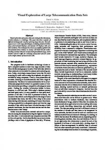
(a) Rhinovirus (1FPN.pdb)

chains

(b) Small ribosomal subunit (1J5E.pdb) at the residue level

(c) Secondary structures in the hemoglobin (1A00.pdb)

(d) Combined volume and isosurface rendering of a dengue virus capsid protein (1R6R.pdb)

Figure 1: Different structures and functions at various LODs can be visualized interactively using TexMol. Figure (a) shows the chains in a rhinovirus colored by the residue they belong to. In Figure (b), we show a small ribosomal subunit at the residue level. Each residue is approximated by a primitive to provide more overall information to the user than that given by a set of atoms. We show the secondary structures of hemoglobin in Figure (c). The four hemes containing the iron atom is shown enclosed between the α helices. A combined volume and isosurface rendering of a virus capsid protein’s hydrophobicity is shown in Figure (d), with the hydrophobic regions shaded yellow and the hydrophilic regions shaded red.

2

R ELATED W ORK

Molecular Modeling and Structural Rendering Numerous modeling schemes have been used to represent and display molecules and their properties on computers [20]. Some models which are structural in nature include the Stick model, the Balland-Stick model, the Wire-Frame model and the Cartoon model. All these in fact are different visual representation of an underlying hierarchical skeletal model of the positions of atoms, bonds, chains, and residues in the molecule. Hence, structural models are designed to represent the primary, secondary, tertiary and quaternary geometric structures of the molecule. Many visualization systems such as RasMol [27], Chime, Protein Explorer [23], PyMol [11], VMD [18], MidasPlus [14], PMV have been created to display the threedimensional structure of a molecule in different styles. A complementary approach to modeling molecule structure is to model properties of the molecule as 3D fields defined over the structural model. This enables either extracting isosurfaces of the fields and their derivatives or examining them using other visualization techniques such as volume rendering and topology graphs. Molecules are thus visualized to have surfaces and occupy volume similar to our perception of surfaces and volume occupancy of macroscopic objects. Molecular Surface Rendering The representation and visualization of molecular surfaces is an important tool in the understanding of fundamental molecular conformation and three dimensional structure. The molecular surface is defined from the van der Waal radii of the individual atoms. Molecular surface models can also represent envelopes of other molecular properties (e.g. electrostatic potential, spin density) [4, 9, 17] and also some molecular interactions in the presence of a solvent (e.g. solvent accessible, solvent contact) [6, 7, 24, 30]. Such surfaces are usually visualized using isosurface or volume renderings of scalar fields along with displays of their gradient vector field or Laplacian scalar field [24, 30, 26, 29]. A vast amount of previous work has covered the representation and visualization of molecular surfaces. Originally proposed by Lee and Richards for use in biochemistry [21], the solvent accessible surface was first extended to computer graphics by Connolly

244

[7, 6] and Max [24]. Much of this preliminary work, along with later extensions [29, 25, 1, 26, 3] focused on finding fast methods of triangulating the solvent-accessible surface. Two prominent obstacles in surface visualization are the correct handling of surface self-intersections to avoid visual artifacts and the high communication bandwidth needed when sending tessellated surfaces to the graphics hardware. Image Based Rendering Techniques Large environments have traditionally been rendered using image based rendering techniques. These techniques usually suffer from popping artifacts and are rigid to changes in lighting. Hence, a renderer must strike the right balance between visual fidelity and performance. View dependent texture mapping, which we employ in TexMol, is commonly used for image-based rendering. In [10], the authors describe an efficient way of implementing such texture mapping through the traditional graphics pipeline. A survey of image based techniques for improving the rendering quality of traditional techniques is given in [5]. Large scale environment visualization through images was shown in [2, 28, 22, 15]. Better depth maintenence was shown in [8, 19]. In [12], an image based rendering algorithm is given which depends on lighting conditions. Using artistic techniques and multiperspective images, [16] present a method of improving the occlusions of objects during motion. Programmable Graphics Hardware The recent interest in image-based rendering has been due in large part to increasingly powerful and increasingly programmable graphics hardware. Cg is a high level Graphics Processing Unit (GPU) programming language developed by NVIDIA that allows users to write custom programs for the vertex and fragment processors in commodity GPU’s. Previous work for practical applications of GPU’s [13] describes the texture-based sphere renderer which was adapted for use in TexMol. Our main contribution for structural rendering is extending previous work on sphere rendering by providing new imposter-based algorithms for cylinders and helices. Our fast, general visualization technique overcomes the bandwidth and artifact problems associated with triangle-based structural rendering. Under imposterbased rendering, each complex geometric primitive is represented by a set of simpler geometric objects, such as a single quadrilateral,

Figure 2: Flexible Chain Complex: Combined volume (through hardware accelerated 3D texture mapping based volume rendering) and imposter rendering, showing the chain together with the high density volumetric regions formed by the functional groups protruding outwards from the chain.

in contrast to the numerous triangles needed to tessellate complex curved primitives. In addition, primitive-primitive intersections under imposter-based rendering are correct on a pixel level with no extra computation, which differs from the expensive clipping algorithms needed to remove artifacts from intersecting sets of triangulations. 3

I NTERNAL R EPRESENTATION

The Flexible Chain Complex (FCC) is our main hierarchical representation for molecular structure. For each chain in the molecule, the chain backbone is stored along with all the residues (amino acids or nucleotides), which are placed at the connection point to the backbone. A helix surrounded by the electron density around the backbone is shown in Figure 2. FCC allows the application to interactively update flexible dihedral angles along the backbone. TexMol also has support for manipulating the rotamer angles within a residue Physical properties of a molecule (e.g. the electron density, electrostatic potential, hydrophobicity, and surface curvatures) can be represented as functions of the atom centers along with the atoms’ properties. Hence the FCC provides a unique skeletal and an implicit volumetric format to efficiently represent structural and functional properties of a molecule. In this paper, we concern ourselves only to visualization and exploration of large FCCs. The FCC can also contain pointers to volume files which explicitly represent properties of the molecule. The volume files are in two formats. Apart from the conventional color index format, we also use the older RGBA format to efficiently render pre-computed structures of the molecule. For example, we could have an RGBA dataset where the molecule is colored per atom according to the color of the residue to which it belongs. The A channel is used to show the dropoff in electron density as distance from the atom center increases. 3.1

Static level-of-detail

The FCC sorts the atoms and superstructures of a molecule into a four-tiered hierarchy which is derived from the biochemical hierarchy used in Protein Data Bank (PDB) files [31]. In this paper, all filenames associated with a molecule refer to the commonly used PDB filename. The following is a top-down view of the hierarchy. • Chain - chain backbone information is stored • Secondary structure - a Helix, a Turn, or a Sheet

(a) Atom level

(b) Residue level with a low blobby factor

Figure 3: LOD volume rendering of a large ribosomal subunit (1JJ2.pdb). The parameter blobbiness controls the spread of the density around a pseudo atom when blurring the chain complex

• Residue - either an amino acid or a nucleotide • Atom - lowest tier, each member is a single atom The hierarchy is constructed from the bottom up, so that every member of the hierarchy, except chains, contains all relevant members from the level immediately below it. For example, each atom only contains itself, since atom is the lowest level of the hierarchy. A residue contains all atoms that are a part of it, while a secondary structure contains all residues that are a part of it. Chains are a unique in that they only contain some of their component members, which will be explained in detail later in this section. TexMol associates each level of the hierarchy with a geometric representation. An atom is represented by a single sphere with the atom’s van der Waal radius. A residue is represented by a minimal single bounding sphere that encloses all of its component atoms. A volume rendering of the atomic and residue level is shown in Figure 3 for a large ribosomal subunit (1JJ2.pdb). In Figure 9, we show the bacteriophage virus’ capsid proteins (1GW7.pdb) at two different levels using different visualization techniques. For secondary structures, sheets and helices are represented by an appropriately-sized geometric sets of cylinders and helices. The orientation, length and radius of these are determined by a least mean square fitting of the central axis to all of the atom centers in either the helix or the sheet’s strand. The third type of secondary structure, turns, are simply represented by their component atoms and bonds along the chain backbone, since turns are usually short atom sequences that feature sharp angles. Not all residues are part of secondary structures, so we simply cluster these otherwise parent-less residues under an imaginary SS NULL group. Chains are represented by including only the atoms in the backbone of the chain. Hence, the chain level does not include any of the functional groups attached to the molecular backbone. Once the hierarchy is created, the user may interactively change the LOD in the hierarchy by picking one of its tiers to visualize. Under static LOD, this selection is applied uniformly across the entire molecular complex (contrast this viewing mode with dynamic LOD explained in Section 4.5). 4

I MPOSTER R ENDERING

The models we encounter in molecular visualization, including the union of balls model, the ball and stick model, the secondary structure model, are composed of regular curved surfaces. The traditional method of rendering these surfaces is to triangulate the surface and render the triangle strips. Due to the large sizes of the data

245

sets we are trying to render, triangulated curved surface rendering is either too computationally expensive or is plagued by visual artifacts. Hence we introduce some new image-based rendering techniques that extend earlier work in sphere rendering. Our main idea comes from the fact that in the programmable graphics hardware, we are allowed to perform a depth replacement at the fragment level. This allows us to render a curved surface with some axis of symmetry without the need for triangulation. NVIDIA’s Cg Tutorial [13] describes a method of rendering spheres with a single quadrilateral, with correct depth and normals under an orthographic projection. In the perspective view, the depth turns out to be an approximation, but still retains good smoothness properties. We extend this work to include other primitives (Figure 4) and apply these new primitives in our molecule visualization. One key advantage of imposter-rendering is per-pixel accurate shading within the resolution of the normal map. Although the resolution of the normal map imposes some limits, the normal map’s resolution may be increased arbitrarily based on the application requirements. In contrast to imposter-based renderers, typical molecular visualizers, such as RasMol and its derivatives, tessellate their geometric primitives, which produces approximate lighting effects and tessellation-related artifacts. Another benefit of imposterrendering is its occurrence near the end of the rendering pipeline, meaning it can be combined with software-based acceleration techniques, such as occlusion culling and adaptive tessellation, to further increase visualizer performance. 4.1

CPK model

The CPK model of a molecule is the geometric union of all of van der Waal radius spheres that correspond to the atoms in the molecule. 4.1.1

Sphere rendering

Texture-based sphere rendering is shown in one of NVIDIA’s Cg Tutorials [13]. We use their method to render spheres in TexMol. The cylinder and helix renderers that will be described in Sections 4.2.1 and 4.3.1, respectively, are extensions of the sphere renderer. 4.2

Ball and Stick model

The ball and stick model is the geometric union of all the atoms and bonds in a molecule, where each atom is represented by a van der Waal radius sphere and each bond is represented by a cylinder that extends between the two atoms that form the bond. Atom radii must be intentionally reduced from the values given in the PDB file in order to make the bonds visible. While the ball and stick model is otherwise very similar to the CPK model, the understated atomic radii places more emphasis on the internal connectivity of the molecule. 4.2.1

Cylinder rendering

The cylinder uses a single quadrilateral as the underlying geometric primitive, along with three texture maps. Unlike a sphere, a cylinder is not rotationally invariant, so its corresponding quadrilateral in clip space reflects the orientation of the actual cylinder in clip space. In our algorithm, we need only one quad to obtain a perfect cylinder, but due to a compiler bug in Cg, we are forced to use two quads. The algorithm for the vertex program and the fragment program is given in Algorithm 1 and Algorithm 2. Our vertex and fragment programs work in GeForce FX cards and beyond. In each of the algorithm descriptions, we have tried to be as brief as possible and also use common abbreviations due to space constraints, without losing any informa-

246

tion. ES, OS refer to EyeSpace and ObjectSpace respectively. MV , MV I, MV P, Pro j, MV PI are the OpenGL ModelView, ModelViewInverse, ModelViewPro jection, Pro jection and the ModelViewPro jectionInverse matrices respectively. By using the vertex and fragment programs in Algorithm 1 and Algorithm 2, we create a single front sided cylinder where the two cylinder bases are not well defined. This design increases performance with no loss in visual quality, since the cylinder bases are always hidden inside spheres in the ball and stick model. In Algorithm 3, we create cylinders with defined bases by ensuring that we have the correct opacity at the ends of the cylinder. This algorithm requires the coordinates of one end point, the axis of the cylinder, and the MVPI matrix. Due to space constraints, we present only the subset of the program that needs to be inserted into the Stick Fragment Program given in Algorithm 2. Figure 4 (b) and (c) depict how quads are transformed in the programmable graphics card into cylinders with proper depth and lighting. Algorithm 1 is still used as the vertex program. Algorithm 1 Stick vertex program 1: Inputs are: [P1, P2, MV, radius, offset, MVI, MVP, Proj] 2: [OS]axis ← P2 − P1 3: [ES]axis ← normalize(MV ∗ [OS]axis) 1 1 = 4: h ← [ES,xy]gradient 2 sqrt(1−[ES]axis.z )

5: [ES, xy]unitAxis ← normalize([ES]axis.y, −[ES]axis.x, 0, 0) 6: [ES, xy]axis = [ES, xy]unitAxis ∗ o f f set ∗ radius 7: if P associated with P1 then 8: if ES.axis.z < 0 then 9: [ES]o f f set ← [ES, xy]o f f set + [ES]axis ∗ h ∗ radius ∗ 10: 11: 12: 13: 14: 15: 16: 17: 18: 19: 20: 21: 22: 23: 24: 25: 26: 27: 28: 29: 30:

4.3

[ES]axis.z else [ES]o f f set ← [ES, xy]o f f set + [ES]axis ∗ h ∗ radius ∗ [ES]axis.z ∗ −1 end if else if ES.axis.z < 0 then [ES]o f f set ← [ES, xy]o f f set + [ES]axis ∗ h ∗ radius ∗ [ES]axis.z ∗ −1 else [ES]o f f set ← [ES, xy]o f f set + [ES]axis ∗ h ∗ radius ∗ [ES]axis.z end if end if [ES]o f f set ← MV I ∗ [ES]o f f set if P associated with P1 then outP ← P1 else outP ← P2 end if HPOS ← MV P ∗ (outP + o f f set) radius ← radius ∗ h [z, w]center ← [MV P[2], MV P[3]].outP [z, w]o f f set ← radius ∗ [Pro j[2], pro j[3]].z Output: [[z,w](center,offset), HPOS, LightVector, Normal, EndPoints, normalized xy position]

Secondary structure representation

We visually represent helix and sheet secondary structures using imposter-based helices and cylinders. Turns are represented by their component atoms and bonds along the backbone since they usually consist of only a handful of atoms.

(a) Sphere rendering from NVIDIA’s depth replace example. We consider two overlapping specular spheres, whose correct appearance is as shown in the rightmost image. We render two rectangles (leftmost image), perform opacity culling (left middle), perform per-pixel normal and lighting evaluation (right middle), and finally replace depth values to obtain the final image (rightmost image).

(b) Four rectangles (two overlapping pairs)

(c) Cylinders after correct opacity, lighting, and depth are assigned

(d) Helices formed from the previous pair of cylinders (new viewpoint).

Figure 4: Imposter rendering of some primitives

Algorithm 2 Stick fragment program 1: Inputs are: [normalized xy position (xy), LightVector, Color, Ambient light] 2: Normal ← Lookup(normalMap, (xy)) 3: Depth ← Lookup(depthMap, (xy)) 4: OutColor = CalculateOut putColor() 5: [z, w] ← Depth ∗ [z, w]o f f set + 1 ∗ [z, w]center 6: OutDepth ← z/w ∗ 0.5 + 0.5 7: Output: [color,opacity,depth]

Algorithm 4 Helix fragment program 1: Inputs are: [refVector, crossRefVector, opacityMap, pitch] 2: if y.inRange() then 3: V ← normalize((IN.xy) − P1 − y ∗ axisDCs) 4: x ← cos−1 (V.(re fVector)) 5: side ← V.crossRe fVector 6: if side < 0 then 7: x ← 2∗π −x 8: end if f mod(y,pitch) 9: y← pitch 10: opacity ← lookup(opacityMap, x, y) 11: end if

4.3.1 Algorithm 3 Cylinder fragment program 1: Inputs are: [P1, axisDCs, length, MVPI, IN.xy] 2: ndcPos ← (IN.x, IN.y, z/w, 1) 3: [OS]P = MV PI ∗ ndcPos 4: y ← axisDCs.(([OS].P − P1).xyz) 5: if y < 0 then 6: opacity ← 0 7: else if y > length then 8: opacity ← 0 9: else 10: opacity ← 1 11: end if

Helix rendering

Helices are composed of two quadrilateral primitives and are an extension to cylinder rendering. We present the fragment program in Algorithm 4, which is the extension which needs to be added to the cylinder fragment program in Algorithm 3. For this fragment program, we need the additional input parameter of a crossRe fVector, which is a vector from one end point of the helix on the axis to any particular point on the helix in object space. Another input needed is an opacity map (a bitmap containing a wrapped diagonal band of the required thickness), which generates the shape of the helix via alpha values. Figure 4(d), shows the two cylinders from Figure 4(c) under the new helix opacity mapping. A slightly different viewpoint is used for the helices to show the correct per-pixel intersections and shading. Figure 5 shows the myoglobin molecule with its helices represented using imposters.

247

Figure 5: Coils showing the presence of α helices in the myoglobin protein. The heme group is shown here with an orange iron atom.

4.3.2

Figure 6: Sets of cylinders representing the strands of two β sheet in a snake toxin protein (1FSC.pdb).

Sheet rendering

Sheets are composed of multiple strands. One method of rendering a sheet is to render the set of strands as cylinders. Hence we use our cylinder rendering when visualizing sheets. The two β sheets of a snake toxin are represented by sets of differently colored cylinders in Figure 6. Multiple cylinders per strand and a color gradient could be used to enhance the folding of the sheet and the strand directions.

4.4

Function-on-surface rendering

We implement embedded surface rendering by extending the previous GPU programs. It is often useful to study the variation of functions on molecular surfaces. These properties can be visualized by accessing two additional custom texture maps in the fragment program. The user can set one texture to the volumetric function, while assigning to the other texture a transfer function map which allows the user to interactively modulate the function being mapped onto the imposter model. One could also implement implicit functions using the fragment program instead of an explicit volumetric grid. In Figure 8, we show the hydrophobicity function being mapped onto the union of balls model of the hemoglobin molecule.

4.5

Dynamic level-of-detail

Dynamic LOD uses the static LOD hierarchy to change regions of the molecule based on the spatial occupancy of these regions from the current viewpoint. Dynamic LOD is currently implemented with bounding spheres on all levels of the hierarchy to limit visually distracting popping when one region switches its LOD. When dynamic LOD is active, molecular regions that occupy fewer pixels on screen are represented with a coarser level in the static hierarchy. This allows the user to see atom-level detail by zooming in, while also being able to capture the overall molecular structure by zooming out. Additionally, realtime scenes with many molecules interacting with one another benefit from dynamic LOD by automatically reducing the geometric complexity of a scene from distant viewpoints, while maintaining the power to explore the scene in detail from other viewpoints.

248

Figure 7: Imposter rendering of the 1.2 million microtubule molecule in two different LODs. The left image shows the atoms rendered as spheres with residue colors. The image in the right shows the residue level of the macromolecule. Rendering such large data sets in high resolution is especially useful for multi tile display and exploration of complex large macromolecules like the microtubule and large viruses.

Figure 8: A synchronized multi-view visualization of two functions of the same hemoglobin dataset. In the left pane, we show the mean curvature on an isosurface of the electron density of the molecule. The red color represents positive mean curvature, while the green shows negative mean curvature and white represents zero mean curvature regions. On the right pane, we have the hydrophobicity function mapped to the imposters, with red representing hydrophilic regions and green representing hydrophobic regions. The hemes groups are shown in black.

Mol Hem

NumAtoms 4770

NumRes 574

Mem (M) 27

Rib

98543

6577

79

Mic

1210410

78210

643

LOD Atom Residue Chain Atom Residue Chain Atom Residue Chain

FPS 28.4 21.3 85.2 7.7 9.5 42.6 1.9 3.6 2.4

Table 1: Performance results for rendering in 800x600 resolution, full screen mode for Hemoglobin (Hem), Ribosome (Rib) and the Microtubule (Mic).

4.6

(a) Imposter rendering of atoms with chain colors

(b) Imposter rendering residues with chain colors

of

(c) Imposter rendering of residues with protein colors

(d) Volume rendering at the residue level with depth coloring

Synchronized multi-view visualization

We define a molecular information view (MI view) to be either a structural representation, a functions-on-surface representation, or a volumetric representation of a molecule. TexMol provides the ability for split-screen visualization that juxtaposes multiple MI views simultaneously. We also allow both synchronous and asynchronous viewing operations to be performed on each view, in effect separating the data model from the viewing model. 5

R ESULTS AND D ISCUSSION

We will first discuss the performance results for running TexMol on a high-end workstation with commodity graphics hardware. Next, we will briefly summarize the various features of the software. 5.1

Performance

TexMol’s performance was measured on a dual Pentium III Xeon 800MHz machine with one gigabyte of memory and an NVIDIA GeForce4 Ti 4200 AGP8X for its GPU. Only one of the dual CPU processors was used during testing. Table 1 shows performance for the hemoglobin, ribosome, and microtubule datasets. The hemoglobin (1A00.pdb) and the large ribosomal subunit (1JJ2.pdb) are taken from the Protein Data Bank [31]. The microtubule data set was donated by Dave Sept and Nathan Baker. The second and third columns list the number of atoms and residues, respectively. The fourth column lists the peak CPU-side memory usage for each experiment. Since a given dataset is always processed the same way to generate the static LOD hierarchy, from which all static LODs can be derived, the CPU-side memory usage is the same regardless of which LOD is selected for rendering. The time taken to parse the files to a hierarchy is considered as a preprocessing step and is not considered here. When we are using dynamic LOD rendering, the time taken to determine the cut in the tree to render is negligible compared to the rendering times. For each trial, the given molecule was rendered across three LODs (fifth column): atom level, residue level, and chain level. The final column lists the frames-per-second performance of the trial. All trials were performed at 800x600 resolution using TexMol’s full-screen mode. The atom LOD sends the most number of geometric primitives to the GPU, so cases where the atom LOD performs worst are vertex limited. We expect this case to occur for extremely dense molecules with high atom counts. The residue LOD provides fewer geometric primitives to the GPU, but residue representations (a conservative bounding ball) take up more screen space than their component atoms. Thus, more fragments are generated in the GPU fragment processor, so cases where the residue LOD perform worst are

Figure 9: The Bacteriophage PRD1 capsid protein (1GW7.pdb). The virus has 34181x60 atoms and 4452x60 residues. Figures (a) (b) and (c) show an imposter view of the virus at the atom level with chain colors and residue level with chain and protein colors. (d) is a depth colored image of the volume representing electron density

fragment limited. Finally, the chain LOD reduces both vertex and fragment load from the atom LOD by 1) rendering only atoms and bonds along the backbone and 2) using primitives that are the size of atoms rather than larger bounding balls. Note, however, that the chain LOD renders more than one geometric primitive per residue, so it still has greater vertex complexity than the residue LOD, which renders exactly one geometric primitive per residue. For the atom LOD, the hemoglobin visualization performs fastest. Since hemoglobin is a relatively small molecule, it stands to reason that it is not vertex limited. On the other hand, the mediumsized ribosome shows signs of being vertex limited, since its performance improves slightly under the residue LOD. Finally, the microtubule, which contains the most vertex information, shows a speedup of about 90% when switching from atom LOD to residue LOD. The slowdown of the microtubule chain LOD is a result of the vertex-limited nature of the rendering, since three atoms are still being drawn per residue. Memory usage for the two larger molecules scales linearly with the size of the molecule, while the hemoglobin memory usage is almost entirely due to the operating overhead of the program (about 20 M). The bacteriophage shown in Figure 9 renders at a peak rate of around 1.2 fps at the full atomic level resolution.

249

5.2

Visualizer features

This section summarizes TexMol’s various features. First, TexMol uses fast imposter-based rendering to render the structural molecular shape at various LODs (Figures 1(a-c), 5, 6). TexMol also renders volumes (using hardware assisted 3D texture maps) independently (Figures 1(d), 3) or in tandem with structure. Structurevolume rendering modes include embedded rendering (Figure 2), function-mapping, and synchronized multi-view (Figure 8). Curvatures and isosurfaces are rendered with traditional geometry. Finally, TexMol can display and animate large molecules at high resolution that were previously intractable. Currently, the massive microtubule complex (Figure 7) animates at a peak rate of 4 fps, and we hope future optimizations lead to interactive rates. 6

C ONCLUSIONS AND F UTURE W ORK

TexMol’s ability to perform a wide range of structural and volumetric rendering concurrently, combined with its aggressive use of programmable graphics hardware, distinguish it from existing molecular visualizers. We hope TexMol will effectively serve the biology community in its ongoing research. In our continuing work, we intend to incorporate visibility and culling techniques to further increase rendering performance. Our ultimate goal is to visualize the 1.2 million atom microtubule dataset at an interactive rate. We are also working on a GPU technique that increases the visual fidelity of volumetric rendering by exploiting symmetry, which is inherent in many large biomolecules, like icosahedral viruses. Future work will also include experimenting with the synchronous multi-view framework in order to discover new ways to visualize the inherent links between molecular structure and molecular function. Acknowledgements The microtubule dataset was provided by Dave Sept and Nathan Baker of Washington University in St. Louis. Several of the virus datasets were provided by Charlie Brooks, Jack Johnson, and Vijay Reddy of the Scripps Research Institute. This research was performed in the Center for Computational Visualization, http://www.ices.utexas.edu/CCV, and supported in part by NSF grants ACI-0220037, CCR-9988357, EIA0325550 and a subcontract from UCSD 1018140 as part of the NPACI project, Interaction Environments Thrust. R EFERENCES [1] Nataraj Akkiraju and Herbert Edelsbrunner. Triangulating the surface of a molecule. Discrete Appl. Math., 71(1-3):5–22, 1996. [2] Daniel Aliaga, Jon Cohen, Andrew Wilson, Eric Baker, Hansong Zhang, Carl Erikson, Kenny Hoff, Tom Hudson, Wolfgang Stuerzlinger, Rui Bastos, Mary Whitton, Fred Brooks, and Dinesh Manocha. Mmr: an interactive massive model rendering system using geometric and image-based acceleration. In Proceedings of the 1999 symposium on Interactive 3D graphics, pages 199–206. ACM Press, 1999. [3] Chandrajit L. Bajaj, Valerio Pascucci, Ariel Shamir, Robert J. Holt, and Arun N. Netravali. Dynamic maintenance and visualization of molecular surfaces. Discrete Applied Mathematics, 127(1):23–51, 2003. [4] Nathan A. Baker, David Sept, Simpson Joseph, Michael J. Holst, and J. Andrew McCammon. Electrostatics of nanosystems: Application to microtubules and the ribosome. Proc. Natl. Acad. Sci., 98:10037– 10041, 2001. [5] Chu-Fei Chang, Zhiyun Li, Amitabh Varshney, and Qiaode Jeffry Ge. Hierarchical image-based and polygon-based rendering for large-scale visualizations. Scientific Visualization, 2001. [6] Michael L. Connolly. Analytical molecular surface calculation. Journal of Applied Crystallography, 16:548–558, 1983. [7] Michael L. Connolly. Solvent-accessible surfaces of proteins and nucleic acids. Science, 221(4612):709–713, 1983.

250

[8] Lucia Darsa, Bruno Costa, and Amitabh Varshney. Walkthroughs of complex environments using image-based simplification. Computers and Graphics, 22(1):25–34, January 1998. [9] Malcolm E. Davis and J. Andrew McCammon. Electrostatics in biomolecular structure and dynamics. Chem. Rev., 90:509–521, 1990. [10] Paul E. Debevec, George Borshukov, and Yizhou Yu. Efficient viewdependent image-based rendering with projective texture-mapping. In 9th Eurographics Rendering Workshop, Vienna, Austria, June 1998. [11] Warren L. DeLano. The pymol molecular graphics system. World Wide Web http://www.pymol.org, 2002. [12] Huong Quynh Dinh, Ronald Metoyer, and Greg Turk. Real-time lighting changes for image-based rendering. IASTED International Conference on Computer Graphics and Imaging, 1998. [13] Randima Fernando and Mark J. Kilgard. The Cg Tutorial: The Definitive Guide to Programmable Real-Time Graphics. Addison-Wesley Pub Co, February 2003. [14] Thomas E. Ferrin, Conrad C. Huang, L. E. Jarvis, and Robert Langridge. The midas display system. Journal of Molecular Graphics, 6:13–27, 1988. [15] David Gotz, Ketan Mayer-Patel, and Dinesh Manocha. Irw: An incremental representation for image-based walkthroughs. ACM Multimedia 2002, 2002. [16] Andrew J. Hanson and Eric A. Wernert. Image-based rendering with occlusions via cubist images. In Proceedings of the conference on Visualization ’98, pages 327–334. IEEE Computer Society Press, 1998. [17] Barry Honig and Anthony Nicholls. Classical electrostatics in biology and chemistry. Science, 268(1144-1149), 1995. [18] William Humphrey, Andrew Dalke, and Klaus Schulten. VMD – Visual Molecular Dynamics. Journal of Molecular Graphics, 14:33–38, 1996. [19] Stefan Jeschke and Michael Wimmer. Textured depth meshes for realtime rendering of arbitrary scenes. In Proceedings of the 13th Eurographics workshop on Rendering, pages 181–190. Eurographics Association, 2002. [20] Andrew R. Leach. Molecular Modelling: Principles and Applications. Addison Wesley, 1996. [21] Byungkook Lee and Frederic M. Richards. The interpretation of protein structures: Estimation of static accessibility. Journal of Molecular Biology, 55:379–400, 1971. [22] Dong Hoon Lee and Soon Ki Jung. Capture configuration for imagebased street walkthroughs. International Conference on Cyberworlds, 03–05:151, December 2003. [23] Eric Martz. Protein explorer: Easy yet powerful macromolecular visualization. Trends in Biochemical Sciences, 27:107–109, February 2002. http://proteinexplorer.org. [24] Nelson Max. Computer representation of molecular surfaces. IEEE Computer Graphics and Applications, pages 21–29, August 1983. [25] Michel F. Sanner, Arthur J. Olson, and Jean-Claude Spehner. Fast and robust computation of molecular surfaces. In Proceedings of the eleventh annual symposium on Computational geometry, pages 406– 407. ACM Press, 1995. [26] Michel F. Sanner, Arthur J. Olson, and Jean-Claude Spehner. Reduced surface: an efficient way to compute molecular surfaces. Biopolymers, 38(3):305–320, March 1996. [27] Roger Sayle and E. James Milner-White. Rasmol: Biomolecular graphics for all. Trends in Biochemical Sciences (TIBS), 20(9):374, September 1995. [28] Gernot Schaufler and Wolfgang Sturzlinger. A three dimensional image cache for virtual reality. Computer Graphics Forum (Eurographics ’96), 15(3):227–235, 1996. [29] Amitabh Varshney and Frederick P. Brooks. Fast analytical computation of richards’s smooth molecular surface. In Proceedings of the 4th conference on Visualization ’93, pages 300–307, 1993. [30] Richard Voorintholt, M. T. Kosters, G. Vegter, Gerrit Vriend, and Wim G. Hol. A very fast program for visualizing protein surfaces, channels and cavities. Journal of Molecular Graphics, 7(4):243–245, December 1989. [31] John Westbrook and Paula M. Fitzgerald. Structural Bioinformatics, pages 161–179. P. E. Bourne and H. Weissig, John Wiley & Sons, Inc., 2003.