and Aya whose love, patience and silence are my shelter whenever it gets hard. To my second wife Limya Abdullah whose love and supplication to Allah were.
�� ����� � �� � � ����� � ��������� � ��� �� ���� �� � ��� � ������� ���� ����� ��� ���!� ��� ���� "� ���� ��""��� ���� ������� �#��� "��� ���� � $�� �" �� �� �� ���� ��� �� � ��� � ��""��� �� � �%� ��� ��� �� � �� � �� �%� ��� � �� �� ��������"���""��� �� ��%� ��� �&�' �������� ����������� ������ � ��� �%� ��� �� ��� �� �"������ ��� ���"��� � �� ���� �� ��� !�� ��� �� � ��� � ��� ���� ��""����&������� ������ ������������ �"� ������""��� ���"���� � ������ ���� �����!� � ��������������� ��� �&�' ��� ������ ��������������
������� ��� �� ����""��� �� ��%� ��� ����� ������������ ���� �� ���������� ������� �"� ��""��� �� � �%� ��� �� ��&�&� ���� ��� �(� ��� � ��� � ��""��� ��
�%� ��� ��&������������� �����"���������"�
� � ������ ��� �)��� ���� � "� �*� ��������� "���������� �� ������*� ��������� �� �������� �� ���� ���� ��* ����$���� !� �����"� ������ ������� ��� �*�����$���� ����� ����"��� ���� * �� ����$�� �� �� �� ����� ��&� �� ���� � �� �"� ����� �� ����� ���� �� ��� �� � ��� � ����� ������ � ������� ���� ��� ���� ���� "� ���� ��""��� ��� ��������+ ��� � ���� �%��� ��� ����� ��� �� ��� � � � �� ���� ��� �� � ���
��""��� �� � �%� ��� �&� ��!��%�� � ��� � #,��� -� ����� �� ��� ���� ����� �� �� �� ������� ������ ��
��������� ���� � ����
,� � �.�� ������ � ������ ��� � ��!�� �� �! � ����� �� �/011&�2����������� �! ��� �� �������� ����� �� �� �� ���� ��"������� 3 ����������"����� ��� ������ � ����4�# �� ����" � �� ���� ��� �/005�� �� �� ������������� ��� �� ���� ����"����-� ��6
���3 ���������� �! � ����� � � �7889&�2���������� � �� � ����� �����"�����&
�����������������
���������� ��
��� ��� � ��� ������� ��������� � �������� ������ �� ��� ���������������� ��� ��
��������� ���� � ���� ���������� ������� ���� ���� ���������
��������� ���� � ����
���������� ������� ���� ���� �� ������ ������� �� ���� �� ����� ���� ���� ������ ��������� ��!���� �!
"� �"��� ��������� �� �# �� �!
���������� ����� � � �������� �� ���� ��� �������������� ���� ���� �������� ������������� � � ���� �������� ��� ������ ���� ������ ������ ����� ��� ���� ����� �� � ���� ��������� ������� ����������������� �� ��� �������������������������
��������� �!�� ��� ��� � � � "���� ��� ������� �� � ��� ������ # ����� ���� �������� ���� ����������� $ ������ ��!%� � ����!� ����� � ������ ��� ��� & ���� ��$ � ���� ' ������ ��� ����� ������� ����� ' ������ ��� ���� (�$�������� �� ��� � ��� '������ ��� ���� # ����%� �������� ���%� )��� � �� ���%� * ������ ���% ' �������� �������� � $ �����������'�������� ����� � �� ������������ +������ ����� �� �� ��� ���� "�� ��%� � ��� ��� �� � ���� ��� &����� ��� ' ������ ��!�����# ����� ���������������� ��� ����������� ����$,��� ����� �������(����� �����������$��������� ��� �������� � � ��� ��� ����������� ����-�� ������� ��� ���� �������� ����. � ����� �� � ���� �������� ��� ������ � ��� ����� ����� ��� � �� ����� � � ���� ��������� ������� ������������� � � �� � � ��� � �� �������� ���������� �� ��������� �!�� �� � "�-��� ���� ���� �������� ��� ������������������ �������� ������(� ���� �� ��� ��%� �� ��� ��� � ����� ����� ����� ��� ��� �� ��� ���� ��� ���������� �� ��� ���� � � � ���� ����� ����� ������ � . �� ���� � � �� ��� � ���%� ����� � � ���%� ������� ���%��� ���� ���%������ ����� ����������� ������$�� ��� �� ��� �� ��� ���������� ���$�������������$ -������� �������������� ��� � �� � � ���� � -� ��� ��� ����� �� �������� ���� ��� ����� �� � � �� ��� ��� �� �� �������� ����������� ����� ��� ������ ������������-� �-��� /�����������/������� ����$$$ ����� �� �� 0��� ���������� ��� 1"��1"#�23.�" ���� ������� ��� ������������������������� ��� ��� ����
4���& �������)��*�5�/� �+) � � � ��� 6��78%�99:::�& ���� ���%������ � �����)��� �2� ������ �;����� ������ �� *��������������� ���������&������ �������� �������� ���� �� � ��������������������� /��-��� ���]`. Numerical techniques other than the dynamic relaxation (DR) method include finite element method (FEM), which is widely used in most of the theoretical analyses of today's research. In a comparison between the dynamic relaxation method and the finite element method, Aalami [10] found that the computer time required for finite element method is eight times greater than that for the dynamic relaxation analysis, whereas storage capacity for finite element analysis is ten times or more than that for DR analysis. This fact is supported by Putcha and Reddy [11], and Turvey and Osman^�>��] ± [��@`, who they noted that some of the finite element �ϱ �
formulations require large storage capacity and computer time. However, if the analysis requires less computations and computer time, then, the dynamic relaxation is considered more efficient than the finite element method. In another comparison Aalami [10] found that the difference in accuracy between one version of finite element and another may reach a value of 10% or more, whereas a comparison between one version of finite element method and DR showed a difference of more than 15%. Therefore, the dynamic relaxation method (DR) can be considered of acceptable accuracy. The only apparent limitation of dynamic relaxation (DR) method is that it can only be applied to limited geometries. However, this limitation is irrelevant to square and rectangular plates and beams which are widely used in engineering applications. The errors inherent in the dynamic relaxation (DR) technique ^>��] ± [��@` include discretization error which is due to the replacement of a continuous function with a discrete function. Also, there is an additional error resulting from the non± exact solution of the discrete equations due to the variations of the velocities from the edges of the plate to the center. The usage of finer meshes reduces the discretization error, but increases the round ± off error due to the large amount of computations involved. For the sake of simplifying and explanation of the DR method, ݑin equation (1.2) is referred to as displacement, and hence the terms ߲ ݑ/ ߲ ݐand ߲ ଶ ݑ/ ߲ ݐଶ are the velocity and acceleration respectively. Accordingly the first and second terms on the right ± hand side are the inertia and damping terms respectively. ߩ And ݇ are the inertia and damping coefficients respectively, and ݐis time. If the velocities before and after the period ο ݐat an arbitrary node in the finite difference mesh are denoted by ሼ߲ݑȀ߲ݐሽିଵ and ሼ߲ݑȀ߲ݐሽ respectively, then using ଵ
finite differences in time, and specifying the value of the function at ሺ݊ െ ሻ, it is ଶ
possible to write equation (1.2) in the following form: �ϲ �
݂ିభ ൌ మ
డ௨
Now ቄ ቅ డ௧
భ మ
ି
ߩ ߲ݑ ߲ݑ ߲ݑ ൜ ൠ െ ൜ ൠ ൨ ݇ ൜ ൠ భ ����������������������������ሺͳǤ͵ሻ ߲ ݐିଵ ߲ ݐି ο ݐ߲ ݐ మ
, which is the velocity at the middle of the time increment, can be
approximated by the mean velocities before and after the time increment,οݐ, which is expressed as follows: ൜
߲ݑ ͳ ߲ݑ ߲ݑ ൠ భ ൌ ൜ ൠ െ ൜ ൠ ൨ ʹ ߲ ݐ ߲ ݐିଵ ߲ ݐି మ
Hence, equation (1.3) can be expressed in the following form as: ݂ିభ ൌ మ
݇ ߲ݑ ߩ ߲ݑ ߲ݑ ߲ݑ ൜ ൠ െ ൜ ൠ ൨ ൜ ൠ െ ൜ ൠ ൨�������ሺͳǤͶሻ ʹ ߲ ݐ ο ݐ߲ ݐ ߲ ݐିଵ ߲ ݐିଵ
Equation (1.4) can then be arranged to give the velocity after the time interval, οݐ: οݐ ߲ݑ ߲ݑ ൜ ൠ ൌ ሺͳ ݇ כሻିଵ ݂ିభ ሺͳ െ ݇ כሻ ൜ ൠ ൨����������ሺͳǤͷሻ ݁ ߲ ݐିଵ ߲ ݐ మ Where: ݇ כൌ
݇οݐ ʹߩ
The displacements at the middle of the next time increment can be determined by integrating the velocity, so that: ߲ݑ ݑାభ ൌ ݑିభ ൜ ൠ ο��������������������������������������������������������ݐሺͳǤሻ ߲ ݐ మ మ The iterative procedure begins at time ݐൌ Ͳ with all initial values of the velocitiesand displacements equal to zero or any other suitable values. In the first iteration, the velocities are obtained from equation (1.5) and the displacements from
�ϳ �
equation (1.6). The boundary conditions are then applied. Subsequent iterations follow the same steps until the desired accuracy is achieved.
1.3 Finite Difference Approximation: ������Ordinary Differential Equations: The values of the interpolating function ݑሺݔሻ in the vicinity of the node ݅ in a non ± uniform or graded mesh shown in figure (1.1) below can be expressed as follows using Taylor's series: ݑሺ݅ ͳሻ ൌ ݑሺ݅ሻ ܲାଵ οݑ�ݔᇱ ሺ݅ሻ
ଷ ସ ܲାଵ �ο ݔଷ ᇱᇱᇱ �ο ݔସ ᇱᇱᇱᇱ ܲାଵ ݑሺ݅ሻ ݑሺ݅ሻ ��������������������������ڮሺͳǤሻ ͵Ǩ ͶǨ
ݑሺ݅ െ ͳሻ ൌ ݑሺ݅ሻ െ ܲ οݑ�ݔᇱ ሺ݅ሻ
െ
ଶ ο ݔଶ ᇱᇱ ܲାଵ ݑሺ݅ሻ ʹǨ
ܲଶ ο ݔଶ ᇱᇱ ݑሺ݅ሻ ʹǨ
ܲସ �ο ݔସ ᇱᇱᇱᇱ ܲଷ �ο ݔଷ ᇱᇱᇱ ݑሺ݅ሻ ݑሺ݅ሻ �����������������������������������ڮሺͳǤͺሻ ͵Ǩ ͶǨ
Figure (1.1) Non ± uniform or graded mesh �ϴ �
Whereݑᇱ ሺ݅ሻ,ݑᇱᇱ ሺ݅ሻ,ݑᇱᇱᇱ ሺ݅ሻ, and ݑᇱᇱᇱᇱ ሺ݅ሻ are the first, second, third, and fourth derivatives of the function ݑሺݔሻ at node݅. ଶ , then subtract the When multiplying equation (1.7) by ܲଶ and equation (1.8) byܲାଵ
latter from the former and rearrange the resulting expression to obtain the function at node ݅ as follows: ݑᇱ ሺ݅ሻ ൌ
ͳ ሺଵሻ ሺଶሻ ሺଷሻ ቂߙ ݑሺ݅ ͳሻ ߙ ݑሺ݅ሻ ߙ ݑሺ݅ െ ͳሻቃ אଵ ������� ሺͳǤͻሻ ο ݔ
Where: ܲାଵ ሺܲ ܲାଵ ሻ
ሺଵሻ
ൌ
ሺଶሻ
ൌെ
െ ାଵ ܲ ܲାଵ
ሺଷሻ
ൌെ
ܲାଵ ሺ ܲାଵ ሻ
ߙ ߙ ߙ
אଵ ൌ െ �ାଵ
ο ݔଶ ᇱᇱᇱᇱᇱ ݅ݑ ������������������������������������������������������������������������ڮሺͳǤͳͲሻ
Multiply equation (1.7) by and equation (1.8) by ାଵ and add them together to obtain the second derivative of the function ݑሺݔሻ at node ݅ as follows: ݑᇱᇱ ሺ݅ሻ ൌ
ʹ ሺସሻ ሺହሻ ሺሻ ቂߙ ݑሺ݅ ͳሻ ߙ ݑሺ݅ሻ ߙ ݑሺ݅ െ ʹሻቃ אଶ � ሺͳǤͳͳሻ ο ݔଶ
Where: ͳ ܲାଵ ሺ ାଵ ሻ
ሺସሻ
ൌ
ሺହሻ
ൌെ
ߙ ߙ
ͳ ܲ ାଵ
�ϵ �
ሺሻ
ߙ
ൌ
ͳ ሺ ାଵ ሻ אଶ ൌ
ܲ െ ܲାଵ ଶ െ � ିଵ ାଵ ଶ ᇱᇱᇱᇱ οݑݔᇱᇱᇱ ݅ െ ο ݅ ݑ ݔ ���ڮሺͳǤͳʹሻ ͵ ͳʹ
If the derivatives of ݂ሺݔሻ which are greater than the third are assumed negligible i.e. the actual function approximates a quadratic function then אଵ and אଶ represent the error in the approximation resulting from replacing the actual function by a quadratic function. The error in the first derivative of the function of equation (1.10) depends on the graded mesh and it is proportional toο ݔଶ . The error in the second derivative of the function, equation (1.12), is proportional to ο ݔଶ for a uniform mesh (i.e.ܲ ൌ ܲାଵ ), and proportional to ο ݔfor a graded mesh (i.e. ܲ ് ܲାଵ ). That is to say the error associated with a graded mesh is greater than that of a uniform mesh with the same number of elements. However, a graded mesh is more flexible than a uniform mesh and it allows closer nodes to be employed in those regions where a higher degree of accuracy is required. When the mesh is uniformܲ ൌ ܲାଵ , and hence: ሺଵሻ
ൌ ߙ
ሺଵሻ
ൌͲ
ሺଵሻ
ൌ ߙ
ሺହሻ
ൌ െͳ
ߙ ߙ ߙ ߙ
ͳ ʹ
ሺସሻ
ൌ
ሺሻ
ൌെ
ͳ ʹ
And therefore, the first and second derivatives, with the error neglected, are as follows: ݀ݑ ͳ ሺ݅ሻ ൌ ሾݑሺ݅ ͳሻ െ ݑሺ݅ െ ͳሻሿ���������������������������������������������ሺͳǤͳ͵ሻ ݀ݔ ʹοݔ � ϭϬ �
݀ଶݑ ͳ ሺ݅ሻ ൌ ଶ ሾݑሺ݅ ͳሻ െ ʹݑሺ݅ሻ ݑሺ݅ െ ͳሻሿ�����������������������������ሺͳǤͳͶሻ ݀ ݔଶ οݔ The first derivative of the function with respect to ݔcan be written also for a uniform mesh as follows with: ݀ݑ ͳ ሺ݅ሻ ൌ ሾݑሺ݅ሻ െ ݑሺ݅ െ ͳሻሿ ݀ݔ οݔ Or ݀ݑ ͳ ሺ݅ሻ ൌ ሾݑሺ݅ ͳሻ െ ݑሺ݅ሻሿ��������������������������������������������������������ሺͳǤͳͷሻ ݀ݔ οݔ 1.3.2 Partial Differential Equations: The first and second derivatives of a function ݑሺݔǡ ݕሻ at an arbitrary node (݅ǡ ݆) shown in figure (1.2) below can be written as follows: ߲ݑ ͳ ሺଵሻ ሺଶሻ ሺଷሻ ሺ݅ǡ ݆ሻ ൌ ቂߙ ݑሺ݅ ͳǡ ݆ሻ ߙ ݑሺ݅ǡ ݆ሻ ߙ ݑሺ݅ െ ͳǡ ݆ሻቃ ߲ݔ ο ݔ ʹ ߲ଶݑ ሺସሻ ሺହሻ ሺሻ ሺ݅ǡ ݆ሻ ൌ ଶ ቂߙ ݑሺ݅ ͳǡ ݆ሻ ߙ ݑሺ݅ǡ ݆ሻ ߙ ݑሺ݅ െ ͳǡ ݆ሻቃ ଶ ߲ݔ οݔ ͳ ߲ݑ ሺଵሻ ሺଵሻ ሺଵሻ ሺ݅ǡ ݆ሻ ൌ ቂߙ ߚ ݑሺ݅ ͳǡ ݆ ͳሻ ߙ ߚ ݑሺ݅ ͳǡ ݆ െ ͳሻ οݔο ݕ ߲ݕ߲ݔ ሺଷሻ ሺଵሻ
ሺଷሻ ሺଷሻ
ߙ ߚ ݑሺ݅ െ ͳǡ ݆ ͳሻ ߙ ߚ ݑሺ݅ െ ͳǡ ݆ െ ͳሻቃ ͳ ሺଵሻ ߲ݑ ሺଶሻ ሺଷሻ ሺ݅ǡ ݆ሻ ൌ ቂߚ ݑሺ݅ǡ ݆ ͳሻ ߚ ݑሺ݅ǡ ݆ሻ ߚ ݑሺ݅ǡ ݆ െ ͳሻቃ ο ݕ ߲ݕ ߲ଶݑ ʹ ሺସሻ ሺହሻ ሺሻ ൌ ଶ ቂߚ ݑሺ݅ǡ ݆ ͳሻ ߚ ݑሺ݅ǡ ݆ሻ ߚ ݑሺ݅ǡ ݆ െ ͳሻቃ ଶ ߲ݕ οݕ Where:
� ϭϭ �
ሺଵሻ
ߙ � ൌ � ሺଶሻ
ߙ � ൌ �
ܲ ܲାଵ ሺܲାଵ ܲ ሻ ܲାଵ െ ܲ ܲ ܲାଵ
ሺଷሻ
ߙ � ൌ � െ ሺସሻ
ߙ � ൌ �
ͳ ܲ ܲାଵ
ሺହሻ
ߙ � ൌ � െ ሺሻ
ߙ � ൌ � ሺଵሻ
ߚ � ൌ � ሺଶሻ
ߚ � ൌ �
ݎ ݎାଵ ሺݎାଵ ݎ ሻ ݎାଵ െ ݎ ݎ ݎାଵ
ሺଷሻ
ሺସሻ
ሺହሻ
ሺሻ
ݎାଵ ݎ ሺݎ ݎାଵ ሻ
ͳ ݎ ݎାଵ
ߚ � ൌ � െ ߚ � ൌ �
ͳ ܲ ܲାଵ
ͳ ܲ ሺ ܲାଵ ሻ
ߚ � ൌ � െ ߚ � ൌ �
ܲାଵ ܲ ሺܲ ܲାଵ ሻ
ͳ ݎ ݎାଵ
ͳ ݎ ሺݎ ݎାଵ ሻ
Where ܲ and ܲାଵ are the ratios of the dimensions of the elements on both sides of the node (݅ǡ ݆) to the average element length all measured in the x ± direction. �ݎ� �And � ϭϮ �
ݎାଵ are the ratios of the dimensions of the elements on both sides of node (݅ǡ ݆) to the average element length all measured in the y ± direction.
݅ െ ͳǡ ݆ ͳ
݅ǡ ݆ ͳ
݅ ͳǡ ݆ ͳ
ݎାଵ οݕ
݅ െ ͳǡ ݆
݅ǡ ݆
݅ ͳǡ ݆
ݎ οݕ
݅ െ ͳǡ ݆ െ ͳ
݅ǡ ݆ െ ͳ
݅ ͳǡ ݆ െ ͳ
ܲ οݔ
ܲାଵ οݔ
Figure (1.2) the first and second derivatives of a two dimensional function ࢛ሺ࢞ǡ ࢟ሻ
When the mesh is uniform i.e. ൌ ܲାଵ �And��ݎ ൌ ݎାଵ , we have: ሺଵሻ
ሺଵሻ
ሺଶሻ
ሺଶሻ
ሺଷሻ
ሺଷሻ
ሺସሻ
ሺସሻ
ሺହሻ
ሺହሻ
ሺሻ
ሺሻ
ߙ ൌ � ߚ ൌ �
ͳ ʹ
ߙ ൌ � ߚ ൌ �Ͳ ߙ ൌ � ߚ ൌ � െ ߙ ൌ � ߚ ൌ �
ͳ ʹ
ͳ ʹ
ߙ ൌ � ߚ ൌ � െͳ ߙ ൌ � ߚ ൌ �
ͳ ʹ
The first and second derivatives of ݑሺݔǡ ݕሻ for a uniform mesh are: � ϭϯ �
߲ݑ ͳ ሺ݅ǡ ݆ሻ ൌ ሾݑሺ݅ ͳǡ ݆ሻ െ ݑሺ݅ െ ͳǡ ݆ሻሿ�������������������������������������������������ሺͳǤͳሻ ʹοݔ ߲ݔ ͳ ߲ݑ ሺ݅ǡ ݆ሻ ൌ ሾݑሺ݅ǡ ݆ ͳሻ െ ݑሺ݅ǡ ݆ െ ͳሻሿ�������������������������������������������������ሺͳǤͳሻ ʹοݕ ߲ݕ ߲ଶݑ ͳ ሺ݅ǡ ݆ሻ ൌ ଶ ሾݑሺ݅ ͳǡ ݆ሻ െ ʹݑሺ݅ǡ ݆ሻ ݑሺ݅ െ ͳǡ ݆ሻሿ�����������������������������ሺͳǤͳͺሻ ଶ ߲ݔ οݔ ߲ଶݑ ͳ ሺ݅ǡ ݆ሻ ൌ ଶ ሾݑሺ݅ǡ ݆ ͳሻ െ ʹݑሺ݅ǡ ݆ሻ ݑሺ݅ǡ ݆ െ ͳሻሿ�����������������������������ሺͳǤͳͻሻ ߲ ݕଶ οݕ ߲ଶݑ ͳ ሺ݅ǡ ݆ሻ ൌ ሾݑሺ݅ ͳǡ ݆ ͳሻ െ ݑሺ݅ ͳǡ ݆ െ ͳሻ ߲ݕ߲ݔ Ͷοݔοݕ െݑሺ݅ െ ͳǡ ݆ ͳሻ ݑሺ݅ െ ͳǡ ݆ െ ͳሻሿ�������������������������������������������������������������
� ϭϰ �
CHAPTER TWO Procedural Steps in Solving Differential Equations Using DR Method
2.1 The Dynamic Relaxation (DR) Program: The DR program performs the following operations: �� Reads data file. �� Computes fictitious densities. �� Computes velocities and displacements. �� Checks stability of numerical computations. �� Checks convergence of solution. �� Checks wrong convergence. Refer to references ^>��] ± [��@` for more information about analysis of rectangular laminated plates in bending.
2.1.1 Numerical Instability: In every iteration, the value of the function at the center of the solution domain or other suitable point is compared with two estimated reference values representing lower and upper bounds of the function at that point. If solution was failed such that the computed value of the function at the specified point did not fall within the prescribed range, the solution is deemed unstable, and therefore iterations are terminated. The damping coefficients are then reduced and the process of iteration is restarted once again. The iterations are repeated several times until stability is reached.
� ϭϱ �
2.1.2 Convergence of DR Solution: Convergence of the dynamic relaxation solution is checked at the end of each iteration by comparing the velocities over the domain with a prescribed value. The procedure is repeated until the solution is deemed converged and consequently the iterative process is terminated.
2.1.3 Convergence to an Invalid Solution: Sometimes DR solution converges to incorrect answer. Check for invalid solution is carried out after the solution has satisfied the convergence criterion explained earlier. In the check procedure the profile of variable is compared with the anticipated profile over the domain. For instance, if the value of the function on the boundaries is zero, and it is known that the function increases from edge to center, and then the solution should follows a similar profile. If the computed profile is different from that, the solution is deemed to be incorrect. When this happens, the solution can hardly be made to converge to the correct answer by altering the damping coefficients and time increment. One should take another look to the boundary conditions and correct them if they are wrong.
2.1.4 Time Increment: Proper time increment is a very important factor for speeding convergence and controlling numerical computations. When time increment is too small, convergence becomes tediously slow; and if it is too large, the solution becomes unstable. Time increment must be less than 1, say, ����
2.1.5 Damping Coefficient: The optimum damping coefficient is that which produces critical motion. When the damping coefficient or coefficients are large, the motion is over ± damped and convergence becomes very slow. When the coefficients are small, the motion is under ± damped and can cause numerical instability. � ϭϲ �
2.2 Solved Examples: In the following examples, the dynamic relaxation (DR) numerical method combined with the finite differences discretization technique is used to solve nonlinear ordinary and partial differential equations. Subsequently a FORTRAN program is developed to generate the numerical results as analytical and/ or exact solutions.
2.2.1 Solution of Ordinary Differential Equation: Example (1): Solve the following ordinary differential equation using the dynamic relaxation (DR) method. ݀ଶݓ � ݍൌ Ͳ���������������������������������������ሺʹǤͳሻ ݀ ݔଶ Where ݍൌ ߨ ଶ �ሺߨݔሻ, and the end conditions are: ݓሺͲሻ ൌ ݓሺͳሻ ൌ Ͳ Note that the exact solution isǣ������ ݓൌ �݊݅ݏሺߨݔሻ.
Solution: Write equation (2.1) in finite difference form as shown below: ݂ൌ
ͳ ሾݓሺ݅ ͳሻ െ ʹݓሺ݅ሻ ݓሺ݅ െ ͳሻሿ ݍሺ݅ሻ ο ݔଶ
The velocities are:
ݓ௧ ሺ݅ሻ ൌ
݂ିభ �οݐ ͳ మ כሺ݅ሻݓ െ ݇ ሺ݅ሻ ͳ ൩ ௧ ିଵ ߩሺ݅ሻ ͳ ݇ כሺ݅ሻ
� ϭϳ �
The values of the function are computed from: ݓሺ݅ሻାభ ൌ ݓሺ݅ሻିభ ݓ௧ ሺ݅ሻ οݐ మ
మ
Now if the region of the problem^0 ±��` is divided into 10 elements, then the end conditions can be expressed as: ݓሺͲሻ ൌ ݓሺͳͲሻ ൌ Ͳ However, in this case and due to symmetry of end conditions, the solution can be obtained over half the domain ^i.e. 0 ±����`. The condition at the symmetry line defined by݅ ൌ ͷ is: ݓሺሻ ൌ ݓሺͶሻ All initial values are set to zero and iterations are started. After each iteration the velocities are compared with a reference of very small value of aboutͳͲି . When all velocities are less than the prescribed value, the process is terminated. The process may be terminated of course when the maximum value of the function (i.e. at center) exceeds certain bounds which indicate that the solution is becoming unstable. These bounds are defined by the inequalitiesͲ ݓ ͷ . After the solution has converged, a further check is made to guarantee that the solution has converged correctly. To facilitate this use is made of the fact that function increases from end to center. In fact this profile is achieved by the converged solution and therefore the solution is considered to be correct. The computer output is listed in table (2.1) below. The solution was converged in 136 iterations. Note the close comparison between the approximate and exact solutions.
� ϭϴ �
Table (2.1) solution of example (1)
ݔ
����
����
����
����
����
( ݓapproximate solution)
������
������
������
������
������
( ݓexact solution)
������
������
������
������
������
The FORTRAN program entitled [Osama 1. FOR] is shown below which is used to solve an ordinary differential equation of example (���) using DR method.
Osama 1. FOR C This program solves an ordinary differential equation using DR C method Real K, KS Dimension X (���� ��Q (���� ��W (���� ��WT (���� Open (unit=5, File='Osama��. Dat', status= 'old') Open (unit = 6, File = 'Osama��. Out', status = 'unknown') Read (5, *) K, DT, RHO, NMAX 8 Format (1x, 'x', 8x, 'w') 9 Format (F4.2, 5x, F6.4) Dx = 0.1 � ϭϵ �
PI = 3.1416 KS = K * DT / (2.0 * RHO) DO 10I = 0���� X (I) = Dx * I Q (I) = (PI ** 2) * sin (PI * X (I)) 10 Continue C Initial Conditions Do 20I = 0���� WT (I)� ���� W (I) = 0.0 20 Continue Do 30N = 1, NMax Do 40 I = 1��� F = ((W (I+1) ± 2.0 * W (I) + W (I ±��))/ (Dx ** 2)) + Q (I) WT (I) = ((1.0 ± KS) * WT (I) + F * DT/ RHO)/ (1.0 + KS) 40 Continue Do 50 I = 1��� W (I) = W (I) + WT (I) * DT 50 Continue C Boundary Conditions � ϮϬ �
W (0) = 0.0 W (10) = 0.0 C Check Instability NL = 0 IF (W (5). GT. 5.0) Then NL = 1 Go To��� Else Continue End if C Convergence Criterion LL = 0 Do 31 I = 0���� IF (WT (I). GT. 0.000001. OR. WT (I). LT. 0.000001) LL = LL + 1 31 Continue IF (LL. GT.�� �Then Go To��� Else Go To���� End if � Ϯϭ �
30 Continue 100 Write (6, *) 'Number of iterations = ', NMAX Write (6, 8) Do 60 I = 0���� Write (6, 9) X (I), W (I) 60 Continue 61 IF (NL. EQ. 1) WRITE (6, *) 'Numerical instability is experienced' Stop End The FORTAN program entitled Osama 2. FOR which is shown below is used to solve ordinary equation of example (���) using exact solution method.
Osama 2. FOR C This program solves an ordinary differential equation using exact solution C method Dimension W������ ��X������ Dx = 0.1 PI = 3.1416 Do 10 I = 0���� X (I) = DX * I � ϮϮ �
10 Continue Do 20 I = 1��� W (I) = sin (PI * X (I)) 20 Continue Write������ 8 Format (1x, 'X', 8x, 'W') Do 30 I = 0���� Write (6, 9) X (I), W (I) 9 Format (1x, F4.2, 5x, F6.4) 30 Continue Stop End
������Solution of Partial Differential Equations: Example (���): Using the dynamic relaxation (DR) method try to solve the following partial differential equation: ߲ଶ߲ ݑଶݑ � ʹߨ ଶ ݑൌ Ͳ�����������������������������������ሺʹǤʹሻ ߲ ݔଶ ߲ ݕଶ Subject to boundary conditions:��ݑሺݔǡ Ͳሻ ൌ Ͳǡ ݑሺݔǡ ͲǤͷሻ ൌ ݊݅ݏሺߨݔሻǡ ݑሺͲǡ ݕሻ ൌ Ͳ, ݑሺͲǤͷǡ ݕሻ ൌ ݊݅ݏሺߨݕሻ � Ϯϯ �
The exact solution is as follows: ݑൌ ሺߨݔሻ �ሺߨݕሻ The Computer output is listed in table (2.2) below. The first row of each set is the approximate solution whereas the second row is the exact value. The solution of this example was converged in 73 iterations.
Solution:
Table (2.2) Solution of example (���)
������
������
������
������
������
������
������
������
������
������
������
������
������
������
������
������
������
������
������
������
������
������
������
������
������
������
������
������
������
������
������
������
������
������
������
������
������
������
������
������
������
������
������
������
������
������
������
������
������
������
������
������
������
������
������
������
������
������
������
������
� Ϯϰ �
������
������
������
������
������
������
������
������
������
������
������
������
�
Equation (2.2) is written in finite differences form as follows: ݂ൌ
ͳ ሾݑሺ݅ ͳǡ ݆ሻ െ ʹݑሺ݅ǡ ݆ሻ ݑሺ݅ െ ͳǡ ݆ሻሿ ο ݔଶ
ͳ ሾݑሺ݅ǡ ݆ ͳሻ െ ʹݑሺ݅ǡ ݆ሻ ݑሺ݅ǡ ݆ െ ͳሻሿ ο ݕଶ
ʹߨ ଶ ݑ The FORTRAN program entitled Osama 3. FOR which is shown below is used to solve ordinary differential equation of example (���) using DR method.
Osama 3. FOR C This program solves a partial differential equation using DR method Real K, KS Dimension X������ ��Y������ ��U������������ ��UT (0:10, 0:10) Open (unit = 5, File = 'Osama 3. Dat', status = 'old') Open (unit = 6, File = 'Osama 3. Out', status = 'unknown') Read (5, *) K, DT, RHO, NMax 8 Format (2x, 'U (I, J)') 9 Format �� (2x, F 6.4)) � Ϯϱ �
NL = 0 DX = 0.1 DY =���� PI = 3.1416 KS = K * DT/ (2.0 * RHO) Do 10 I = 0��� X (I) = DX * I 10 Continue Do 11 J = 0��� Y (J) = DY * J 11 Continue Do 20 I = 0��� Do 20 J = 0��� U (I, J) = 0.0 UT (I, J) = 0.0 20 Continue Do 30 N = 1, NMax Do 40 I = 1��� Do 40 J = 1��� F = (U (I+1, J) ±����� �U (I, J) + U (I-1, J))/ (DX ** 2) + (U (I, J+1) � Ϯϲ �
±����� �U (I, J) + U (I, J-�))/ (DY ** 2) + 2.0 * PI ** 2 * U (I, J) UT (I, J) = ((1.0 ± KS) * KS) *UT (I, J) + F * DT / RHO) / (1.0 + KS) 40 Continue Do 50 I = 1��� Do 50 J = 1��� U (I, J) = U (I, J) + UT (I, J) * DT 50 Continue C Boundary conditions Do 41 I = 0��� U (I, 0) = 0.0 U (I, 5) = sin (PI * X (I)) 41 Continue Do 42 J = 0��� U (0, J) = 0.0 U (�, J) = sin (PI * Y (J)) 42 Continue C Check Instability IF (U (5, 5). GT. ��� Then NL = 1 Go To��� � Ϯϳ �
Else Continue End if C Convergence Criterion LL = 0 Do 31 I = 0��� Do 31 J = 0��� IF (UT (I, J). LT. 0.000001) LL = LL + 1 31 Continue If (LL. GT. 0) Then Go To 30 Else Go To 100 End if 30 Continue ����Write (6, *) 'Number of iterations = ', NMax Write (6, 8) Do 60 I = 0��� Write (6, 9) (U (I, J), J = 0.5) 60 Continue � Ϯϴ �
61 If (NL. EQ. 1) write (6, *) 'Numerical instability is experienced' Stop End The FORTRAN program entitled Osama �. FOR is illustrated below which is used to solve a partial differential equation of example (���) using the exact or analytical solution.
Osama �. FOR C This program solves an ordinary differential equation C using exact solution method Dimension U (0:10, 0:10), X (0:10), Y (0:10) DX = 0.1 DY ���� PI = 3.1416 Do 10 I = 0���� Do 20 J = 0���� X (I) = DX * I Y (J) = DY * J 10 Continue Do 20 I = 1���
� Ϯϵ �
U (I, J) = sin (PI * X (I)) * sin (PI * Y (J)) 20 Continue Do 30 I = 0��� WRITE (6, 9) (U (I, J), J = 0��� � Format �� (1 X, F 6.4)) 30 Continue Stop END
Example (���): Solve the following system of partial differential equations over a square domain bounded by Ͳ ݔ ͳ and Ͳ ݕ ͳusing DR method.
߲ଶݑ ߲ଶݒ ߲ଶݑ ߲ݓ ʹ െݑ ൌ Ͳۗ ߲ ݔଶ ߲ ݕ߲ ݕ߲ݔଶ ߲ݔ ۖ ۖ ݀ଶݒ ߲ଶݑ ߲ଶݒ ߲ݓ ʹ െݒ ൌ Ͳ �����������������ሺʹǤ͵ሻ ݀ ݔଶ ߲ ݕ߲ ݕ߲ݔଶ ߲ݕ ۘ ۖ ߲ݑ ߲ݒ ߲ଶݓ ߲ଶݓ ۖ � � � � � � � ݍ ൌ Ͳ ߲ ݕଶ ߲ݔ ߲ݕ ߲ ݔଶ ۙ ଵ
Where ݍൌ �ߨ ቀߨ ଶ ቁ ሺߨݔሻ ��ሺߨݕሻ� ଶ
Solution: The boundary conditions are as given in the next figure (i.e. figure (2.3)). Note that the differential equations are satisfied by the following solutions: � ϯϬ �
ͳ ݑൌ
ሺߨݔሻ �ሺߨݕሻ ͺ ͳ ݒൌ ሺߨݔሻ
�ሺߨݕሻ ͺ ݓൌ
ͳ Ͷߨ ଶ ሺߨݔሻ �ሺߨݕሻ ͺߨ
Figure (2.3) Boundary Conditions of Example (2.3)
Write equation (���) in finite difference form: ݂ଵ ൌ
ͳ ሾݑሺ݅ ͳǡ ݆ሻ െ ʹݑሺ݅ǡ ݆ሻ ݑሺ݅ െ ͳǡ ݆ሻሿ ο ݔଶ
ͳ ሾݒሺ݅ ͳǡ ݆ ͳሻ െ ݒሺ݅ ͳǡ ݆ െ ͳሻ െ ݒሺ݅ െ ͳǡ ݆ ͳሻ ݒሺ݅ െ ͳǡ ݆ െ ͳሻሿ Ͷοݔοݕ
ͳ ሾݑሺ݅ǡ ݆ ͳሻ െ ʹݑሺ݅ǡ ݆ሻ ݑሺ݅ǡ ݆ െ ͳሻሿ െ ݑሺ݅ǡ ݆ሻ ο ݕଶ
� ϯϭ �
݂ଶ ൌ
ͳ ሾݓሺ݅ ͳǡ ݆ሻ െ ݓሺ݅ െ ͳǡ ݆ሻሿ ʹοݔ
ͳ ሾݒሺ݅ ͳǡ ݆ሻ െ ʹݒሺ݅ǡ ݆ሻ ݒሺ݅ െ ͳǡ ݆ሻሿ ο ݔଶ
ͳ ሾݑሺ݅ ͳǡ ݆ ͳሻ െ ݑሺ݅ ͳǡ ݆ െ ͳሻ െ ݑሺ݅ െ ͳǡ ݆ ͳሻ ݑሺ݅ െ ͳǡ ݆ െ ͳሻሿ Ͷοݔοݕ
ͳ ሾݒሺ݅ǡ ݆ ͳሻ െ ʹݒሺ݅ǡ ݆ሻ ݒሺ݅ǡ ݆ െ ͳሻሿ െ ݒሺ݅ǡ ݆ሻ ο ݕଶ
݂ଷ ൌ
ͳ ሾݓሺ݅ǡ ݆ ͳሻ െ ݓሺ݅ǡ ݆ െ ͳሻሿ ʹοݕ
ͳ ሾݓሺ݅ ͳǡ ݆ሻ െ ʹݓሺ݅ǡ ݆ሻ ݓሺ݅ െ ͳǡ ݆ሻሿ ο ݔଶ
ͳ ͳ ሾݑሺ݅ ͳǡ ݆ሻ െ ݑሺ݅ െ ͳǡ ݆ሻሿ ሾݒሺ݅ǡ ݆ ͳሻ െ ݒሺ݅ǡ ݆ െ ͳሻሿ ʹοݕ ʹοݔ
ͳ ሾݓሺ݅ǡ ݆ ͳሻ െ ʹݓሺ݅ǡ ݆ሻ ݓሺ݅ǡ ݆ െ ͳሻሿ ݍሺ݅ǡ ݆ሻ ο ݕଶ
Compute the velocities: ݑ௧ ሺ݅ǡ ݆ሻ ൌ
ͳ ݂ଵ οݐ ൝ሾͳ െ ݇௨ כሺ݅ǡ ݆ሻሿݑ௧ ሺ݅ǡ ݆ሻିభ ൬ ൰ ൡ ߩ ͳ ݇௨ כሺ݅ǡ ݆ሻ మ ௨ ሺ݅ǡ ݆ሻ ାభ మ
ݒ௧ ሺ݅ǡ ݆ሻ ൌ
݂ଶ οݐ ͳ ൝ሾͳ െ ݇௩ כሺ݅ǡ ݆ሻሿݒ௧ ሺ݅ǡ ݆ሻିభ ൬ ൰ ൡ ߩ௩ ሺ݅ǡ ݆ሻ ାభ ͳ ݇௩ כሺ݅ǡ ݆ሻ మ మ
ݓ௧ ሺ݅ǡ ݆ሻ ൌ
݂ଷ οݐ ͳ כ ሺ݅ǡ ݆ሻሿݓ௧ ሺ݅ǡ ݆ሻିభ ൬ ൝ሾͳ െ ݇௪ ൰ ൡ כሺ݅ǡ ݆ሻ ߩ௪ ሺ݅ǡ ݆ሻ ାభ ͳ ݇௪ మ మ
Compute the values of�ݑሺ݅ǡ ݆ሻ,ݒሺ݅ǡ ݆ሻ and�ݓሺ݅ǡ ݆ሻ, from the following equations: � ϯϮ �
ݑሺ݅ǡ ݆ሻାభ ൌ ݑሺ݅ǡ ݆ሻିభ ݑ௧ ሺ݅ǡ ݆ሻ �οݐ మ
మ
ݒሺ݅ǡ ݆ሻାభ ൌ ݒሺ݅ǡ ݆ሻିభ ݒ௧ ሺ݅ǡ ݆ሻ �οݐ మ
మ
ݓሺ݅ǡ ݆ሻାభ ൌ ݓሺ݅ǡ ݆ሻିభ ݓ௧ ሺ݅ǡ ݆ሻ �οݐ మ
మ
Apply the boundary conditions. If the domain is divided into 100 dements: 10 elements in the ݔ± direction and 10 elements in the ݕ± direction, then: ݓሺͲǡ ݆ሻ � ൌ �ݓሺͳͲǡ ݆ሻ ൌ Ͳ ͳ ݑሺͲǡ ݆ሻ ൌ � െݑሺͳͲǡ ݆ሻ ൌ � ߨ݊݅ݏሺ݆�οݕሻ ͺ ݒሺͲǡ ݆ሻ � ൌ �ݒሺͳͲǡ ݆ሻ ൌ Ͳ ݓሺ݅ǡ Ͳሻ � ൌ �ݓሺ݅ǡ ͳͲሻ ൌ Ͳ ݑሺ݅ǡ Ͳሻ � ൌ �ݑሺ݅ǡ ͳͲሻ ൌ Ͳ ͳ ݒሺ݅ǡ Ͳሻ ൌ � െݒሺ݅ǡ ͳͲሻ ൌ � ߨ݊݅ݏሺ݆�οݔሻ ͺ After each iteration check is made on the convergence and stability of the solution. The solution is considered converged when the velocities all over the domain is less thanͳͲି . The criterion for instability is set by taking the bounds on ݓas: Ͳ ݓ ͷ . When solution has converged a further check is made for convergence to an invalid answer. One must remember to exploit symmetry if it exists, a facility provided by the computer program listed next. In this example the solution can be obtained over one quarter of the domain using the following boundary conditions: ݓሺǡ ݆ሻ ൌ ݓሺͶǡ ݆ሻ ൌ Ͳǡ ݒሺǡ ݆ሻ ൌ ݒሺͶǡ ݆ሻ ൌ Ͳǡ ݑሺǡ ݆ሻ ൌ െݑሺͶǡ ݆ሻ ൌ Ͳ � ϯϯ �
ݓሺ݅ǡ ሻ ൌ ݓሺ݅ǡ Ͷሻ ൌ Ͳǡ ݒሺ݅ǡ ሻ ൌ ݒሺ݅ǡ Ͷሻ ൌ Ͳǡ ݑሺ݅ǡ ሻ ൌ ݑሺ݅ǡ Ͷሻ ൌ Ͳ The FORTRAN program entitled Osama �. FOR is shown below which is used to solve a system of partial differential equations of example (���) using DR method.
Osama 5. FOR C This program solves a system of partial differential equations C using DR method Real K, KS Dimension X������ ��Y������ ��U������������ , V������������ , W������������ , UT (0:10, 0:10), VT (0:10, 0:10), WT (0:10, 0:10), Q (0:10, 0:10) Open (unit = 5, File = 'Osama �. Dat', status = 'old') Open (unit = 6, File = 'Osama �. Out', status = 'unknown') Read (5, *) K, DT, RHO, NMAX 8 Format (1X, 'U (I, J)') ���Format (� (1X, F 6.4)) 9 Format (1X, 'V (I, J)') ���Format (� (1X, F 6.4)) 12 Format (1X, 'W (I, J)') ���Format (� (1X�����)) NL = 0 � ϯϰ �
DX = 0.1 DY = 0.1 PI = 3.1416 KS = K * DT/ (2.0 * RHO) Do 10 I = 0���� X (I) = DX * I 10 Continue Do 11 J = 0���� Y (J) = DY * J 11 Continue Do 20 I = 1���� Do 20 J = 1���� Q (I, J) = PI * ((PI ** 2) + 0.� � �sin (PI * X (I)) * sin (PI * Y (J)) 20 Continue Do 30 I = 0���� Do 30 J = 0���� U (I, J) = 0.0 UT (I, J) = 0.0 V (I, J) = 0.0 VT (I, J) = 0.0 � ϯϱ �
W (I, J) = 0.0 WT (I, J) = 0.0 30 Continue Do 40 N = 1, NMAX Do 50 I = 1��� Do 50 J = 1��� F � = ((U (I+1, J) ± 2.0 * U (I, J) + U (I-1, J)) / (DX ** 2)) + ((V (I+1, J+1) ± V (I+1, J-1) ±V (I-1, J+1) +V (I-1, J-�)) / (4.0 * DX * DY)) + ((U (I, J+1) ± 2.0 * U (I, J) + U (I, J-� � �� (DY ** 2)) ± U (I, J) + ((W (I+1, J) ± W (I-1, J)) / (2.0 * DX)) F 2 = ((V (I+1, J) ±����� �V (I, J) + V (I-1, J)) / (DX ** 2)) + ((U (I+1, J+1) ± U (I+1, J-1) ±U (I-1, J+1) +U (I-1, J-�)) / (4.0 * DX * DY)) + ((V (I, J+1) ±����� �V (I, J) + V (I, J-�)) / (DY ** 2)) ± V (I, J) + ((W (I, J��) ± W (I, J-�)) / (2.0 * DY)) F � = ((W (I+1, J) ±����� �W (I, J) + W (I-1, J)) / (DX ** 2)) + ((U (I+1, J) ± U (I-1, J))/ (2.0 * DX)) + ((V (I, J+1) ± V (I, J-�)) / (����* DY)) + ((W (I, J+1) ±����� �W (I, J) + W (I, J-�)) / (DY ** 2))+Q (I, J) UT (I, J) = ((1.0 ± KS) * UT (I, J) + F1 * DT / RHO) / (1.0 + KS) VT (I, J) = ((1.0 ± KS) * VT (I, J) + F2 * DT / RHO) / (1.0 + KS) � ϯϲ �
WT (I, J) = ((1.0 ± KS) * WT (I, J) + F3 * DT / RHO) / (1.0 + KS) 50 Continue Do 60 I = 1��� Do 60 J = 1��� U (I, J) = U (I, J) + UT (I, J) * DT V (I, J) = V (I, J) + VT (I, J) * DT W (I, J) = W (I, J) + WT (I, J) * DT 60 Continue C Boundary Conditions Do 41 J = 0���� W (0, J) = 0.0 W (10, J) = 0.0 U (0, J) = 0.125 * sin (PI * Y (J)) U (10, J) = -0.125 * sin (PI * Y (J)) V (0, J) = 0.0 V (10, J) = 0.0 41 Continue Do 42I� ������ W (I, 0 � ���� W (I, 10 � ���� � ϯϳ �
U (I, 0) = 0.0 U (I, 10) = 0.0 ��ሺ ǡ Ͳሻ � ൌ �ͲǤͳʹͷ� �� כሺ� � ��� כሺ ሻ�ሻ� V (I, 10) = -0.125 * sin (PI * X (J)) 42 Continue C Check Instability IF (W (5���). GT. 5.0) Then NL = 1 Go To��� Else Continue End if C Convergence Criterion LL = 0 Do 31 I = 0���� Do 31 J = 0���� IF (UT (I, J). LT. ����������OR. VT (I, J). LT. 0.000001. OR. WT (I, J). LT. 0.000001)) LL = LL + 1 31 Continue IF (LL. GT. 0) Then � ϯϴ �
Go To��� Else Go To���� End if 40 Continue ����Write (6, *) ' Number of iterations = ', NMAX Write������ Do 70 J = 0��� Write (6, 13) (U (I, J), I = 0���) 70 Continue Write������ Do 80 J = 0��� Write�������) (V (I, J), I = 0���) 80 Continue Write������� Do 90 J = 0��� Write (6, 15) (W (I, J), I = 0.5) 90 Continue 61 IF (NL. EQ. 1) write (6, *) ' Numerical instability is experienced' Stop � ϯϵ �
END
Osama 6. FOR The FORTRAN program entitled Osama �. FOR is shown below which is used to solve a system of partial differential equations of example (���) using exact solution. C This program solves a system of partial differential equations C using exact solution Dimension X (0:10), Y (0:10), U (0:10, 0:10), V (0:10, 0:10), W (0:10, 0:10) � Format (�X, 'U (I, J)') 8 Format (6 (2X, F 6.4)) ���Format (2X, 'V�����J)¶ ��Format (� (�X, F 6.4)) 14 Format (�X, 'W (I, J)') ���Format (� (�X, F ���)) DX = 0.1 DY = 0.1 PI = 3.1416 Do 10 I = 0��� X (I) = DX * I 10 Continue
� ϰϬ �
Do 11 J = 0.� Y (J) = DY * J 11 Continue Do 20 I = 1��� Do 20 J = 1��� U (I, J) = 0.125 * cos (PI * X (I)) * sin (PI * Y (J)) V (I, J) = 0.125 * sin (PI * Y (I)) * cos (PI * Y (J)) W (I, J) = ((1.0 + 4.0 * PI **2)/ (8.0 * PI)) * sin (PI * X (I)) * sin (PI * Y (J)) 20 Continue Write (6, 7) Do 30 J = 0��� Write (6, 8) (U (I, J), I = 0���) 30 Continue Write (6, 13) Do 40 J = 0��� Write (6, 9) (V (I, J), I = 0���) 40 Continue Write (6, 14) Do 50 J = 0��� Write (6, 12) (W (I, J), I = 0���) � ϰϭ �
Stop END
� ϰϮ �
CHAPTER THREE Conclusions
The basics of this book stand on the ordinary and partial differential equations, which value the price of an option by using dynamic relaxation (DR) techniques. The study of partial differential equations in complete generality is a vast undertaking. As almost all of them are not possible to solve analytically we must rely on numerical methods, and the most popular ones are the finite differences methods coupled with dynamic relaxation techniques. With this book we do not intend to become experts in few hours in order to solve differential equations numerically, but develop both intuition and technical strength required to survive when such a problem needs to be solved. In comparison with other numerical methods, the dynamic relaxation technique has its own strengths and weaknesses. The advantages of the DR method are that: (a) the method has a simple algorithm so that it will simplify programming; (b) the formulation is explicit. Therefore, the required memory is less than other techniques; (c) this method has a high ability in intense nonlinear behaviors. The disadvantages and limitations of the DR methods are summarized as that: (a) in general, the method is unstable and needs some additional conditions to guarantee numerical stability; (b) the iterations of the method are done in constant load. This causes some issues in limit points; (c) in nonlinear analysis, with gentle stiffening; the number of iterations is much more in comparison with other techniques. In the dynamic relaxation technique, the static equations of the differential equations system will be converted to dynamic equations. Then the inertia and damping terms are added to all of these equations. The iterations of the dynamic relaxation technique can then be carried out in the following procedures: � ϰϯ �
�� Set all initial values of variables to zeros. �� Compute the velocities. �� Compute the displacements. �� Apply suitable boundary conditions for the displacements. �� Compute the required variables. �� Apply the appropriate boundary conditions for the required variables. �� Check if the convergence criterion is satisfied, if it is not repeat the steps from � to� �� A Dynamic Relaxation (DR) program based on finite differences has been developed for the analysis of one dimensional and two dimensional ordinary and partial differential equations. Finite differences coupled with dynamic relaxation method (DR) have been developed. FORTRAN programs have been compiled which they yielded results for a wide range of examples written and solved with the dynamic relaxation numerical method. These results were found to be in good agreement with those available in the literature of this book and solved using the exact analytical solution. Therefore, a wide spectrum of comparisons between the dynamic relaxation numerical solutions and analytical exact solutions have been undertaken to demonstrate the accuracy of the DR program. The outcomes of these comparisons are found to be of acceptable accuracy. These results show that the convergence of the DR solution depends on several factors including the following:
1. Time increment: It is a very important factor for speeding convergence and controlling numerical computations.
2. Damping coefficients: Is that which produces critical motion.
� ϰϰ �
3. Boundary conditions: It is clear that the type of boundary condition is an important factor in determining the values of variables throughout the system.
4. Mesh size: As the mesh size is reduced, the variables will be stable and smooth in values.
5. Discretization of elements: Finer meshes reduce the discretization error, but at the same time increase the round off error due to the large number of calculations involved.
6. Fictitious densities: They are used to evaluate the values at the far edges of the differential system. The fictitious densities vary from point to point over the system as well as for each iteration. Therefore, to stabilize the solution and to improve the convergence of the numerical computations fictitious densities must be applied.
With my best wishes Osama Mohammed Elmardi Suleiman Mechanical Engineering Department Faculty of Engineering & Technology Nile Valley University Atbara, Sudan
� ϰϱ �
Bibliography: [1] Rushton K.R., 'Large deflection of variable thickness plates', International Journal of Mechanical Sciences, Vol. 10, (1968), PP. (723 ±���� � [2] Cassel A.C. and Hobbs R.E., 'Numerical Stability of Dynamic Relaxation Analysis of Nonlinear Structures', International Journal for Numerical Methods in Engineering, Vol. 35, No. 4, (1966), PP. (1407 ±����� � [3] Day A.S., 'An Introduction to Dynamic Relaxation', the Engineer, Vol. 219, No. 5688, (1965), PP. (218 ±���� � [4] S.P. Timoshenko, 'History of Strength of Materials', McGraw ± Hill, New York,� ����� � [5] J. R. H. Otter, 'Computations for prestressed concrete reactor pressure vessels using dynamic relaxation', Nuclear Structural Engineering 1, (1965), PP. (61 ±��� � [6] L.C. Zhang, 'Dynamic relaxation solution of elastic circular plates in large deflection under arbitrary axisymmetric loads', The third "�.4" Scientific Conference of Peking University, Peking University, Beijing, P.R. China, May (1987). [7] S.W. Keyetal., 'Dynamic relaxation applied to quasi ± static, large defection, inelastic response of axisymmetric solids', In Nonlinear Finite Element Analysis in Structural Mechanics (Edited by W. Wunderlich et al.), Springer, New York, (1981), PP. (585 ±���� � [8] G.T. Lim and G.J. Turvey, 'On the elastic ± plastic large deflection response of stocky annular steel plates', Computer and structure, 21, (1985), PP. (725 ±���� � [9] P.A. Frieze et al., 'Application of dynamic relaxation to the large deflection elasto ± plastic analysis of plates', Computer and structure, 8, (1978), PP. (301 ±���� � [10] Aalami B., 'Large Deflection of Elastic Plates under Patch Loading', Journal of Structural Division, ASCE, Vol. 98, No. ST 11, (1972), PP. (2567 ±����� � � ϰϲ �
[11] Putcha N.S. and Reddy J.N., 'A refined Mixed Shear Flexible Finite Element for the Non ± Linear Analysis of Laminated Plates', Computers and Structures, Vol. 22, No. 4, (1986), PP. (529 ±���� � [12] Turvey G. J. and Osman M. Y., 'Large Deflection Analysis of Orthotropic Mindlin Plates', Proceedings of the 12 th Energy ± Resources Tech. Conference and Exhibition, Houston, Texas, (1989), PP. (163 ±���� � [13] Turvey G.J. and Osman M.Y., 'Large Deflection effects in Antisymmetric Cross ± Ply Laminated Strips and plates', I.H. Marshall, Composite Structures, Vol. 6, Paisley College, Scotland, Elsevier science publishers, (1991), PP. (397 ±���� � [14] Turvey G. J. and Osman M.Y., 'Elastic Large Deflection Analysis of Isotropic Rectangular Mindlin Plates', International Journal of Mech. Sciences, Vol. 22,� ����� � PP. (1 ±��� � [15] M. Mehrabian, M.E. Golma Kani, 'Nonlinear Bending Analysis of Radial Stiffened Annular Laminated Plates with Dynamic Relaxation Method', Journal of Computers and Mathematics with Applications, Vol. 69, (2015), PP. (1272 ±����� � [16] M. Huttner, J. Maca, P. Fajman, 'The Efficiency of Dynamic Relaxation Method in Static Analysis of Cable Structures', Journal of Advances in Engineering Software, ����� � [17] Javad Alamatian, 'Displacement Based Methods for Calculating the Buckling Load and Tracing the Post Buckling Regions with Dynamic Relaxation method, Journal of Computers and Structures, Vols. 114 ± 115, (2013), PP. (84 ±��� � [18] M. Rezaiee Pajand, S. R. Sarafrazi, H. Rezaiee, 'Efficiency of Dynamic Relaxation Method in Nonlinear Analysis of Truss and Frame Structures', Journal of Computers and Structures, Vol. 112 ± 113, (2012), PP. (295 ±���� �
� ϰϳ �
>��@�Kyoung Soo Lee, Sang Eul Han, Taehyo Park, 'A simple Explicit Arc ± Length Method using Dynamic Relaxation Method with Kinetic Damping', Journal of Computers and Structures, Vol. 89, Issues 1 ± 2, (2011), PP. (216 ±���� � [20] J. Alamatian, 'A New Formulation of Fictitious Mass of the Dynamic Relaxation Method with Kinetic damping', Journal of Computers and Structures, Vol. 90 ±����� ����� , PP. (42 ±��� � [21] M. Rezaiee Pajand et al., 'A New Method of Fictitious Viscous Damping Determination for the Dynamic Relaxation Method', Journal of Computers and Structures, Vol. 89, Issues 9 ± 10, (2011), PP. (783 ±���� � [22] B. Kilic, E. Madenci, 'An Adaptive Dynamic Relaxation Method for Quasi ± Static Simulations using the Peridynamic Theory', Journal of Theoretical and Applied Fracture Mechanics, Vol. 53, Issue 3, (2010), PP. (194 ±���� � [23] C. Douthe, O. Baverel, 'Design of Nexorades or Reciprocal Frame Systems with the Dynamic Relaxation Method', Journal of Computers and Structures, Vol. 87, Issue 21 ± 22, (2009), PP. (1296 ±����� � [24] M. Mardi Osama, 'Verification of Dynamic Relaxation Method in the Analysis of Isotropic, Orthotropic and Laminated Plates using Large Deflection Theory', University of Shendi Journal, Volume 10, January (2011), PP. (31 ±��� � [25] Osama Mohammed Elmardi, 'Verification of Dynamic Relaxation (DR) Method in Isotropic, Orthotropic and Laminated Plates using Small Deflection Theory', International Journal of Advanced Science and Technology, Volume 72, Issue 4, (2014), PP. (37 ±��� � [26] Osama Mohammed Elmardi, 'Validation of Dynamic Relaxation (DR) Method in Rectangular Laminates using Large Deflection Theory', International Journal of Advanced Research in Computer Science and Software Engineering, Volume 5, Issue 9, September (2015), PP. (137 ±���� � � ϰϴ �
[27] Osama Mohammed Elmardi, 'Nonlinear Analysis of Rectangular Laminated Plates Using Large Deflection Theory', International Journal of Emerging Technology and Research, Volume 2, Issue 5, September ± October (2015), PP. (26 ±� �� � [28] Osama Mohammed Elmardi, ' Bibliography and Literature Review on Buckling of Laminated Plates ', International Journal of Science and Engineering (EPH), Volume 2, Issue 8, August (2016), PP. (104 ±����). >��] Javier Rodriguez Garcia, 'Numerical study of dynamic relaxation methods and contribution to the modeling inflatable life jackets', University of Brestagne Sud, ����� � >��] L.C. Zhang and T.X. Yu, 'Modified Adaptive Dynamic Relaxation Method and its Application to Elastic ± Plastic Bending and Wrinkling of Circular Plates', Computers and Structures, Volume 33, No. 2, (1989), PP. (609 ±���� � >��] L.C. Zhan and T. X. Yu, 'Application of mechanics of plasticity to the bending forming of beams and plates (in Chinese Language), Journal of Applied Science, 1, (1988), PP. (1 ±��� ��
� ϰϵ �
Author � Osama Mohammed Elmardi Suleiman was born in Atbara, Sudan in 1966. He received his diploma degree in mechanical engineering from Mechanical Engineering College, Atbara, Sudan in 1990. He also received a bachelor degree in mechanical engineering from Sudan University of Science and Technology ± Faculty of Engineering in 1998, and a master degree in solid mechanics from Nile Valley University (Atbara, Sudan) in 2003. He contributed in teaching some subjects in other universities such as Red Sea University (Port Sudan, Sudan), Kordofan University (Obayied, Sudan), Sudan University of Science and Technology (Khartoum, Sudan) and Blue Nile University (Damazin, Sudan). In addition, he supervised more than hundred and fifty under graduate studies in diploma and B.Sc. levels and about fifteen master theses. He is currently an assistant professor in department of mechanical engineering, Faculty of Engineering and Technology, Nile Valley University. His research interest and favourite subjects include structural mechanics, applied mechanics, control engineering and instrumentation, computer aided design, design of mechanical elements, fluid mechanics and dynamics, heat and mass transfer and hydraulic machinery.�He also works as a consultant and technical manager of Al ± Kamali workshops group for small industries in Atbara old and new industrial areas. � ������� �
� ϱϬ �