CZ-377 01 Jindrichuv Hradec, Czech Republic email: {pudil, mikovair, malecm}@fm.vse.cz. ABSTRACT. Image inpainting as a means of substituting missing ...
Proceedings of the 10th IASTED International Conference SIGNAL AND IMAGE PROCESSING (SIP 2008) August 18-20, 2008 Kailua-Kona, HI, USA
TEXTURE ORIENTED IMAGE INPAINTING BASED ON LOCAL STATISTICAL MODEL ´ a´ and Miroslav Malec Pavel Pudil and Irena Mikov Faculty of Management Prague University of Economics Jaroˇsovsk´a 1117/II CZ-377 01 Jindˇrich˚uv Hradec, Czech Republic email: {pudil, mikovair, malecm}@fm.vse.cz
Jiˇr´ı Grim and Petr Somol Department of Pattern Recognition Institute of Information Theory and Automation Academy of Sciences of the Czech Republic P.O.BOX 18, CZ-18208 Prague 8, Czech Republic email: {grim, somol}@utia.cas.cz ABSTRACT Image inpainting as a means of substituting missing image parts can become difficult when the image is textured. In this paper we apply a local statistical model of the source color image with the aim to predict missing texture regions. We have shown in a series of papers that textures can be modeled locally by estimating the joint probability density of spectral pixel values in a suitably chosen observation window. For the sake of image inpainting we estimate the joint multivariate density in the form of a Gaussian mixture of product components. The missing image region is inpainted iteratively by step-wise prediction of the unknown spectral values.
be difficult. Although some parts of search of the suitable textures can be done automatically, the corresponding software solutions are usually time consuming [2]. In addition, it would be necessary to distinguish between textured and “structured” areas and choose a suitable technique for each type of background. In our paper we investigate an original approach to textured image inpainting based on modeling using a mixture of Gaussian components of special type. After the model is obtained, it is used for sequential prediction of the missing parts. We assume it is known which pixels or regions are to be substituted. The method makes use of a recently proposed approach to texture modeling based on estimating the statistical texture properties locally [10], [11], [12]. We estimate the joint probability density of the spectral pixel values within a small observation window in the form of a Gaussian mixture of product components. Using a data set obtained by pixelwise shifting of the observation window we can estimate the mixture parameters by means of the EM algorithm. The distribution mixture model describes the statistical properties of the image by fitting the mixture components to the typical patches as they occur in the observation window. The selection of the most typical window patch representants is optimally controlled by the underlying log-likelihood criterion. Finally, the prediction of missing parts is easily achievable via computing conditional probability distributions. In the inpainting phase the prediction formula automatically chooses the best continuation of the image at the boundary of missing parts. The paper is organized as follows. In Sec. 2 we describe the properties of local statistical model. The principle of image inpainting by prediction is subject of Sec. 3. Sec. 4 describes the computational experiments and finally we summarize the results in the Conclusion Section.
KEY WORDS Image Restoration, Image Inpainting, Color Texture Prediction, Local Texture Model, Gaussian Mixtures, EM Algorithm.
1. Introduction Image inpainting has become a well established field in computer graphics with many potential applications, including repair of missing or damaged image parts, (semi-) automatic retouching of objects in images and videos, but also bandwidth preservation in image transfer etc. Numerous contributions to the field have appeared since the seminal works of Bertalamio at al. [1], [2] and others [3], [4] with very good results achieved on a range of various image types. The techniques employed range from isophote line detection and reconstruction [2], [5] over geometric partial differential equations [6], global image statistics [7] to wavelets [8]. Most of the work cited above focuses on extrapolation of the surrounding image region into the missing area. Yet some of the more problematic cases are images containing textured regions, where many successful inpainting methods produce too apparent non-texture like patches. There are successful alternative techniques to fill a missing area with a selected texture [3], [9], [2] but they have some disadvantages. Usually the user has to select the texture piece to be copied into the missing area and, in case of regions including several background textures, the inpainting may
623-053
2. Local Statistical Model The local statistical model has been proposed originally for textures but the technique is applicable to arbitrary images as well. In the following we consider a digitized color image, possibly containing textured regions, described by a matrix of vector variables where each pixel specifies three
15
RGB spectral values I
we maximize the corresponding log-likelihood function 1 X log P (x) = L= |S|
J
Z = [z ij ]i=0 j=0 , z ij = (zij1 , zij2 , zij3 ) ∈ R3 .
x∈S
Here i, j correspond to row and column indices respectively. In order to describe local properties of the image we assume a square observation window with cut-off corners (cf. [13]) to simply emulate the ”ideal” circular shape. Given an observation window centered at a position (i, j) we denote x(i, j) = x = (x1 , x2 , . . . , xN ) ∈ X , X = R
X 1 X = log [ wm F (x|µm , σ m )] |S| x∈S
by means of the well-known EM iteration equations [11] : E-step:
N
(m ∈ M, n ∈ N , x ∈ S)
wm F (x|µm , σ m ) q(m|x) = P , m∈M j∈M wj F (x|µj , σ j )
the vector of spectral values of the window pixels in a fixed arrangement, i.e. for each pixel there are three spectral values xn . In each position we treat the window contents (image patch) x as an observation of a random vector and assume that the statistical properties of the variables xn can be described by a multivariate probability density. For this purpose we approximate the unknown density function in the form of Gaussian mixture X P (x) = wm F (x|µm , σ m ), x ∈ X , (1)
(5)
M-step: 0
wm =
1 X q(m|x), |S|
(6)
x∈S
X 1 xn q(m|x), x∈S q(m|x)
0
µmn = P
(7)
x∈S
X 1 x2n q(m|x). q(m|x) x∈S x∈S (8) Here the apostrophe denotes the new parameter values in each iteration. Let us remark that the difficult implementation points of EM algorithm (e.g., the existence of local maxima of the likelihood function and the related problem of a proper choice of the initial parameter values) are less relevant if the sample size is sufficiently large as in our case. Considering problem dimensionality N ≈ 101 − 102 , number of components M ≈ 102 and the number of samples K ≈ 106 , we may expect numerous local maxima of the log-likelihood function (4) but, according to our experience, the various mixture estimates resulting from various initialization points are of comparable quality and are usable equally well for our task. It should be noted that the log-likelihood criterion (4) implicitly assumes the data vectors x ∈ S to be independent and identically distributed according to the probability density P (x). Unfortunately, this condition is not guaranteed in case of the shifting window because the respective image patches overlap in different positions of the window. For this reason the data vectors x ∈ S correspond only to a specific “trajectory” in the sample space X and therefore the data set S may have bad sampling properties (cf. [10], [11], [12]). However, in case of image inpainting, this aspect shows to be less relevant since in the prediction formula the estimated distribution is applied mainly to the original “training” data which correspond to the known parts of the image. 0
0
(σmn )2 = −(µmn )2 + P
m∈M
M = {1, 2, . . . , M }, N = {1, 2, . . . , N }. Here M and N denote the index sets of components and variables respectively, wm are probability weights and F (x|µm , σ m ) denote the mixture components defined as products of univariate Gaussian densities [11], [12]: Y F (x|µm , σ m ) = fn (xn |µmn , σmn ), (2) n∈N
� � (xn − µmn )2 1 exp − . fn (xn |µmn , σmn ) = √ 2 2σmn 2πσmn It can be seen that the diagonal form of covariance matrices of the Gaussian densities (2) does not imply the restrictive assumption of independence of variables in x. With a large number of components (in our case M ≈ 102 ) the Gaussian mixture (1) is capable of describing rather general probability density functions and becomes similar to the well known non-parametric Parzen estimate. Let us recall that, choosing the Parzen window function in the form (2), we can guarantee the Parzen estimate to be asymptotically unbiased and consistent when the smoothing parameters σn approach zero with the increasing sample size. From the computational point of view the product components (2) avoid the risk of ill-conditioned covariance matrices and simplify the evaluation of marginal densities [cf. later Eq. (12)]. The standard way to estimate mixtures is to use the EM algorithm [11], [14]. By using the “image patch” data set S obtained by pixel-wise shifting the observation window through the original texture image S = {x(1) , . . . , x(K) }, x(k) ∈ X , (K = |S|),
(4)
m∈M
3. Local Image Prediction The statistical description of the local image properties by the Gaussian density mixture (1) naturally suggests the possibility of local image prediction. Let us suppose that, at a
(3)
16
given position of the observation window, some part of the image patch is known. Denoting xC = (xn1 , xn2 , . . . , xnl ) ∈ XC , XC = R|C|
by increasing the prediction step to about half the window size, the synthesized textures became more stable and more realistic. This effect is probably due to the limited accuracy of the estimated mixture model. A greater prediction step requires only lower dimensional marginals of the estimated mixture which are probably less biased by the limited quality of the estimated mixture P (x). In case of image inpainting the situation is principally different. The missing parts of the image are usually restricted in size and therefore only a few prediction steps are sufficient to “propagate” the information from boundary image regions into the missing area. For this reason the problem of instability is of considerably less importance. In all our computational experiments we have obtained the best results when predicting one pixel at a time. Another problem point in texture synthesis is the proper choice of window size. On one hand the window should be large enough to reproduce the low-frequency details of the texture image, on the other hand the resulting dimension of the estimated probability density should be as small as possible. Problem dimensionality quickly increases as a function of window size and therefore the variability of observed image patches increases quickly in the same image. Although large, the available data set (|S| ≈ 106 ) may easily occur to be insufficient to estimate the underlying multivariate mixture model reliably if the window size is too large. Moreover, from the computational point of view the EM estimation of complex Gaussian mixtures can become unbearably time-consuming even for moderate window size. In the following section we show which settings proved applicable.
(9)
C = {n1 , n2 , . . . , nl } ⊂ N the subvector of all given pixel variables, we can estimate the remaining missing pixel values xn , n ∈ (N \ C), by means of the conditional densities pn|C (xn |xC ) = =
X
Pn,C (xn , xC ) = PC (xC )
(10)
Wm (xC )fn (xn |µmn , σmn ).
m∈M
Here
wm F (xC |µm , σ m ) Wm (xC ) = P . j∈M wj F (xC |µj , σ j )
(11)
are the conditional weights given xC and Y F (xC |µm , σm ) = fn (xn |µmn , σmn ), xC ∈ XC n∈C
(12) denotes the marginal component functions corresponding to the subspace XC . Note that the simple plug-in formula (10) is formally enabled by a simple evaluation of the marginal densities Pn,C (xn , xC ) and PC (xC ). For a fixed position of the observation window the formula (10) can be applied to any missing variable xn , n ∈ N \ C. Thus, by computing the conditional expectation Z X E{xn } = xn pn|C (xn |xC )dxn = Wm (xC )µmn ,
4. Computational Experiments
m∈M
(13) we can estimate even single missing spectral values in the window. In our experiments we have used the computationally more efficient random sampling instead of the conditional expectation formula (13). As the dimension of the space X is relatively high (N ≈ 102 ), the mixture components F (x|µm , σm ) are nearly non-overlapping. For this reason the conditional weights (11) have nearly binary properties and we can consider in Eq. (13) only the term with the highest conditional weight Wm (xC ) without any essential loss of accuracy. In this way the part of the observation window to be inpainted can be actually covered by the corresponding component means µmn of the most “suitable” component. The newly obtained grey levels xn can be later used to upgrade the conditional weights Wm (xC ) in the next prediction step. In our previous experiments with texture synthesis we have used initially a pixel-wise left-to-right and topto-down shifting of the observation window. In this way we tried to supply maximum information in the prediction formula (13) but the process was rather instable. After several prediction steps the texture synthesis often failed completely with a noisy texture image as a result. Surprisingly,
Image inpainting based on local statistical model provides a unified “compromise” solution that treats both the textured and “structured” image areas in the same way without the necessity to choose a suitable technique for each type of background. The estimated mixture components optimally fit to the typical variants of the window patches and the corresponding means are then used to reconstruct the missing parts of the image. In view of Sec. 2 the selection of the typical component means is optimally controlled by the log-likelihood function (4) which is known to be a powerful criterion to fit the parametric mixture model to the available data. In the inpainting phase the prediction formula (12) merely identifies the piece of background at a given position of the window and chooses the best component mean to extrapolate the surrounding area. In this way local statistical model provides a unified highly specific solution to the problem of differently textured and structured areas of the image at the level of the window patch. In order to illustrate the properties of the proposed method we have chosen two 1280 × 960 images. The first image is composed of four different types of textures (cf. Fig. 1). It can be seen that the model based prediction removes the superimposed text successfully while reproduc-
17
Figure 1. Example of image inpainting I.
18
Figure 2. Example of image inpainting II.
19
ing the underlying textures with only minor wrinkles. The second example (cf. Fig. 2) illustrates the method in case of an outdoor scene picture containing various textured and structured parts. Also in this case the inpainting was relatively successful, at least in the sense of achieving visually unobtrusive reconstruction. The varying background of the regularly positioned black holes provides excellent illustration of the prediction capabilities of the model. In both experiments the local statistical model had been estimated from the source damaged image. The only parameters to be specified by the user are the window size (we chose a square window of 7 × 7 pixels with cut-off corners, i.e. N = 111 = 3 ∗ (7 ∗ 7 − 4 ∗ 3)) and the number of mixture components (M ≈ 500 ÷ 700). Training samples have been obtained from positions where the window does not interfere with damaged areas. The training set thus consisted of roughly 800000 samples in the first example and 1150000 in the second example. The EM algorithm has been stopped automatically by the relative increment threshold � = 10−3 , i.e., by the condition ∆L/L < 10−3 . The resulting 15–20 iterations required about several hours of CPU time (AMD Athlon 64). In the inpainting phase we have proceeded iteratively. In each iteration we made the prediction only at window positions with only one missing pixel. The actual inpainting procedure needed about 10–50 iterations taking several minutes of CPU time.
painting, Proc. Conf. on Computer Vision and Pattern Recognition (CVPR’01), Vol. 1, IEEE Computer Society, 2001 [2] M. Bertalmio, G. Sapiro, V. Caselles & C. Ballester, Image inpainting, Computer Graphics (SIGGRAPH), 2000, 417–424 [3] H. Igehy & L. Pereira, Image replacement through texture synthesis, Proc. Int. Conf. on Image Processing (ICIP ’97), Vol. 3, IEEE, Washington, 1997 [4] C. Ballester, M. Bertalmio, V. Caselles, G. Sapiro & J. Verdera, Filling-in by joint interpolation of vector fields and gray levels, IEEE Trans. on Image Processing, 10(8), 2001, 1200–1211 [5] J. Wu & Q. Ruan, Object Removal By Cross Isophotes Exemplar-based Inpainting, Proc. 18th Int. Conf. on Pattern Recognition (ICPR’06), Vol. 3, 2006, 810–813 [6] M. Bertalmio, Strong-continuation, contrast-invariant inpainting with a third-order optimal PDE, IEEE Trans. on Image Processing, 15(7), 2006, 1934–1938 [7] A. Levin, A. Zomet &Y. Weiss, Learning How to Inpaint from Global Image Statistics, Proc. Conf. on Computer Vision and Pattern Recognition (CVPR’03), Vol. 1, IEEE Computer Society, 2003 [8] T.F. Chan, J. Shen & H.M. Zhou, Total Variation Wavelet Inpainting, J. Math. Imaging Vis., 25(1), Kluwer, 2006, 107–125
5. Conclusion In this paper we propose a color image inpainting algorithm based on statistical model of local textural properties. We describe the statistical dependencies between the spectral pixel values in a suitably chosen observation window by a multivariate Gaussian mixture with product components. We estimate the mixture parameters by means of the EM algorithm from source color image patch data obtained by pixelwise shifting the observation window through the source color texture image. The estimated mixture components optimally represent the typical variants of the window patches and the corresponding means are then used to reconstruct the missing parts of the image. The image inpainting based on local statistical model provides a unified solution to the problem instead of choosing specific methods for different types of image areas to fit either textures or “geometric” structures.
[9] M. Bertalmio, L. Vese, G. Sapiro & S. Osher, Simultaneous Structure and Texture Image Inpainting, Proc. Conf. on Computer Vision and Pattern Recognition (CVPR’03), Vol. 2, IEEE Computer Society, 2003 [10] J. Grim & M. Haindl, Texture Modelling by Discrete Distribution Mixtures, Computational Statistics and Data Analysis, 41(3-4), 2003, 603–615 [11] M. Haindl, J. Grim, P. Somol, P. Pudil & M. Kudo, A Gaussian mixture-based color texture model, Proc. 17th IAPR Int. Conf. on Pattern Recognition, IEEE, Los Alamitos, 2004, 177–180 [12] M. Haindl, J. Grim, P. Pudil & M. Kudo, A Hybrid BTF Model Based on Gaussian Mixtures, Texture 2005. Proc. 4th Int. Workshop on Texture Analysis, IEEE, Los Alamitos, 2005, 95–100
Acknowledgements ˇ This research was supported by the projects: GACR No. 102/07/1594 and No. 102/08/0593, 2C06019 ZIMOLEZ ˇ and MSMT 1M0572 DAR.
[13] J. Grim, P. Somol, M. Haindl & P. Pudil, A statistical approach to local evaluation of a single texture image, Proc. 16th Annual Symposium PRASA 2005, University of Cape Town, 2005, 171–176
References
[14] G.J. McLachlan & D. Peel, Finite Mixture Models, John Wiley & Sons, New York, 2000
[1] M. Bertalmio, A.L. Bertozzi & G. Sapiro, NavierStokes, Fluid Dynamics, and Image and Video In-
20