The Algorithm of Continuous Optimization Based on the ... - MDPI
Recommend Documents
Nov 30, 2016 - The kidneys are a pair of bean-shaped organs that lie on either side of the spine in the lower middle of the ... leads (I, II, III) derive signals from the left arm (LA), the right arm (RA) and the left leg (LL). ...... In: Silviu F, e
May 11, 2014 - The Scientific World Journal. Nest. Food. Food. (a) Ant colony position distribution in the initial moment. Nest. Food. Food. (b) Ant colony ...
Jan 2, 2018 - on Sperm Fertilization Procedure (MOSFP) Method .... Network modeling is a process to simplify and represent different kinds ... In this section, we will summarize a few studies that use a wide variety ...... node (ps) of accessing the
Dec 11, 2015 - The advantages and disadvantages of the three algorithms are ...... S. Extended Kalman Filter for wireless LAN based indoor positioning. Decis.
Jun 8, 2017 - In this paper, we focus on a routing optimization algorithm, which solves .... colony system, and introduces pheromone swapping operation to make it ..... In the environment of simulation software platform, this paper selects the ...
Dec 22, 2018 - users, actualize differentiated business networks, and achieve a larger comprehensive evaluation value of the path compared with other algorithms. .... into multiple segments, each of which is identified by a segment identifier. .....
2Graduated Student, Email: [email protected]. 3Graduated ... algorithm where best solution of each iteration is directly copied to the next iteration to improve performance of .... optimization, while API may also be used for discrete ...
Mar 25, 2013 - [17] Kennedy J. and Eberhart R. C., (1995). ... [28] Yang X. S. and Deb S., (2010). ... [37] Deb K., Pratap A., Agarwal S., Mayarivan T., (2002).
Page 1 ... The presented technique is inspired by social behavior of fire- ... intelligence optimization technique is based on the assumption that solution of.
Classification; Sequential Forward Floating Search; Optimization. I. INTRODUCTION .... used to embed the bio-inspired algorithm (SSO) into the web service.
Mar 25, 2013 - We validate the proposed approach using a selected subset of test functions and then apply it to solve design optimization benchmarks. We will ...
Abstract. Firefly algorithm is an evolutionary computing model that is based on behavior of the fireflies in nature. Two of the parameters of this algorithm are.
Genetic algorithms are stochastic search approaches based on randomized operators, such as selection, crossover and mutation, inspired by the natural ...
search to find the solutions for optimization problems. We investigate two ... Keyword small-world phenomenon, optimization algorithm, function optimization, 0-1.
swarm algorithm called the Social Spider Optimization (SSO) is proposed for ... Computational intelligence has emerged as powerful tools for information pro-.
Local search operator for BSWA. Î. Long-range search operator for BSWA k. Iteration ...... [1] Daniel G. 1997. Principles ... [6] Russell C., Eberhart, Y. Shi. 2001.
Page 1. AbstractâHeuristic optimization techniques have became very popular ... Index TermsâBat algorithm, continuous optimization, exploration and ...
Aug 29, 2016 - algorithm that can obtain efficient packet forwarding in a variable network topology becomes a key interest domain. For networks that consist of ...
Aug 27, 2018 - However, in indoor environments, satellite signals are easily occluded and ... of a log-normal shadowing radio propagation model for the estimationof the ..... 2 - xm. 2 + y1. 2 - ym. 2 + d1. 2 - dm. 2 x2. 2 - xm. 2 + y2. 2 - ym.
Aug 29, 2016 - ... same place, such as passengers on the same train and employees in ..... process, the role of the stranger gradually reduced, while the role of ...
Jul 2, 2018 - Unlike the platform-based inertial navigation system, the SINS and the RSINS .... SINS or RSINS for ships and submarines, the fine alignment is ...
The Continuous Genetic Algorithm. 51. Now that you are convinced (perhaps) that the binary GA solves many opti- mization problems that stump traditional ...
where the values of the variables are continuous and you want to know them ... has its precision limited by the binary representation of variables, using float-.
The Algorithm of Continuous Optimization Based on the ... - MDPI
Aug 25, 2016 - Tomsk State University of Control Systems and Radioelectronics, 40 Lenina ... physical, biological, or social systems consisting of a considerable .... Cellular automata are abstract models for systems consisting of a large ...
SS symmetry Article
The Algorithm of Continuous Optimization Based on the Modified Cellular Automaton Oleg Evsutin *, Alexander Shelupanov, Roman Meshcheryakov, Dmitry Bondarenko and Angelika Rashchupkina Tomsk State University of Control Systems and Radioelectronics, 40 Lenina Prospect, Tomsk 634050, Russia; [email protected] (A.S.); [email protected] (R.M.); [email protected] (D.B.); [email protected] (A.R.) * Correspondence: [email protected]; Tel.: +7-3822-90-01-11 Academic Editors: Ka Lok Man, Yo-Sub Han and Hai-Ning Liang Received: 20 March 2016; Accepted: 22 August 2016; Published: 25 August 2016
Abstract: This article is devoted to the application of the cellular automata mathematical apparatus to the problem of continuous optimization. The cellular automaton with an objective function is introduced as a new modification of the classic cellular automaton. The algorithm of continuous optimization, which is based on dynamics of the cellular automaton having the property of geometric symmetry, is obtained. The results of the simulation experiments with the obtained algorithm on standard test functions are provided, and a comparison between the analogs is shown. Keywords: continuous optimization; metaheuristics; cellular automata
1. Introduction The problems of optimization in different application areas often appear when choosing the best variant out of a majority of possible ones is required. Nowadays, many methods for solving similar tasks are known. It is possible to divide them into two big classes: deterministic and stochastic. The deterministic methods let us guarantee the optimality of a solution with the given accuracy, while the stochastic methods in the common case do not give us information about the accuracy of the found solution. Nevertheless, they do show a relatively high effectiveness in optimizing complex objective functions in practice. Consequently, the methods of optimization, which appertain to the second class, are also called heuristic. The major part of the stochastic methods is based on the search for the optimal solution which imitates the behavior of the complicated physical, biological, or social systems consisting of a considerable number of intercommunicate homogeneous elements [1–4]. This article suggests drawing upon the cellular automaton, which is an object of discrete mathematics characterized by different symmetry properties, both in geometrical and algebraic meaning. In our case, we used the cellular automaton which has the property of geometrical symmetry on the level of local rule of evolution. It is necessary to note that there have appeared a variety of research works concerning hybridization of the cellular automata mathematical apparatus with different metaheuristics. In papers [5,6], cellular automata are used together with genetic algorithms. Traditionally, chromosomes which are operated by genetic algorithms are represented in the form of irregular sets of binary vectors. In [5] they are recorded in cells of the two-dimensional cellular automaton, and during crossing over each chromosome takes genetic material from neighbors from the Moore neighborhood. The mutation is realized in the usual way. An additional operation is the shuffle of chromosomes in the lattice for improvement of genetic material interchange. Paper [6] is devoted to an inverse problem. In that paper the cellular automaton serves to model the groundwater allocation, and a genetic algorithm is applied for the adjustment of the model. In this case, states of a lattice of the cellular automaton are coded by means of chromosomes of the genetic Symmetry 2016, 8, 84; doi:10.3390/sym8090084
www.mdpi.com/journal/symmetry
Symmetry 2016, 8, 84
2 of 18
algorithm, and the ultimate goal is the deriving of an optimum state. In article [7] by the same author, the results of a similar research are presented, the research differing only in the harmony search application. In some other papers, cellular automata are merged with the algorithms of optimization which refer to swarm intelligence. So, in paper [8], a modified ant colony algorithm is presented, in which a many-dimensional search space is considered as a cellular structure. For this purpose, a quantity of vectors is picked from the search space, and each of the vectors is called a cell. The points of the space standing apart from the given cell, when this distance does not exceed a certain value, organize a neighborhood. A cell with its neighborhood is called a region. In the given paper, cellular evolution is perceived as the motion of ants in the search space and the ants realize optimum search in each region and can pass from one region to another. In [9] the cellular automata approach is applied to improve the particle swarm optimization algorithm. For this purpose, the authors of the paper introduce the concept of particle neighborhood which is perceived as an assemblage of particles of the swarm closest to the given particle. This concept is used for modification of the particles velocity calculation equation: instead of a randomly chosen element of a swarm, the best particle of the neighborhood is introduced. Besides, a special feature of the given research consists in specificity of the considered problem of optimization. The offered in [9] hybrid algorithm is used for optimization of truss structures. A similar direction is presented in papers [10–12]. The solution of structural optimization problems is also considered. The cellular automaton serves for modelling of the structure which is necessary to optimize. Optimization consists in obtaining such configuration of the cellular automaton which will correspond to the best parameters of the modelled structure. Thus, in this case cellular automata are simultaneously applied as an optimization means and as a modelling environment. The approach used in [13] for improvement of the membrane algorithm is similar to the approach used in [5] with reference to the genetic algorithm. The computing model on which the membrane algorithm is based represents a membrane system. Its principal components are membrane structure, reaction rules, and multisets. In [13], the elements of a multiset contained in the separately taken elementary membrane are represented in the form of a two-dimensional lattice, and at renovation of a state of each element, states of the neighboring elements from the Moore neighborhood are considered. However, in the research provided, cellular automata are used indirectly only, mainly by transmitting their peculiar principle of local interaction to the basic metaheuristic model, which does not bring out the best of the given mathematical apparatus in solving optimization problems. The principle of local interaction is one of the basic parameters of the cellular automaton: the state of all cells renovates at each step of the automaton development, depending on the state of their neighbors [14]. Consequently, in the majority of the papers indicated, the use of the cellular automaton is, in the variety of the solutions under study, limited to introducing a notion of the neighborhood area and to considering vectors from the neighborhood area while a new state of each vector containing the solution options is being calculated. Unlike the previous papers, in paper [15] cellular learning automata are used. In the given paper, they are merged with an artificial fish swarm algorithm, imitating the behavior of a fish swarm in search of food. As a base computing model, using a one-dimensional learning cellular automaton consisting of D cells according to the dimensionality of the optimization problem being solved is suggested. Each cell of such automaton represents a separate n-dimensional learning automaton, associated with an artificial fish swarm responsible for optimization of one measurement of the objective function. Development of the given paper is an original algorithm presented in [16]. It is based on integration of differential evolution and a computing model of learning cellular automata which does not refer to nature-inspired models. In more details, the given algorithm will be considered in the following section of this article. Our paper develops the application of the cellular automata as the mathematical tool to the problem of continuous optimization. As distinct from the well-known approaches, it is suggested to
Symmetry 2016, 8, 84
3 of 18
use the dynamics of the cellular automata for the immediate optimum search in the solution space. Also added is the modification of the classic model of the cellular automaton on the basis of which the optimization algorithm is being formulated and studied. 2. Methods 2.1. Optimization on the Basis of Learning Cellular Automata In the given section we will consider the optimization method offered in [16] in more detail. This method is based on cellular learning automata and differential evolution algorithm (CLA-DE). The CLA-DE method differs from the analogs considered in introduction in that it is not a modification of any known metaheuristics. The differential evolution declared in the title is used not as a basis, but only for improvement of the base calculation model. The basis of the CLA-DE method is the computing model of cellular learning automata which merges cellular automata with learning automata. A learning automaton is an adaptive decision-making system situated in an unknown random environment. This system learns the optimal action through repeated interactions with its environment. The learning is as follows: at each step, the learning automaton selects one of its actions according to its probability vector and performs it on the environment. The environment evaluates the performance of the selected action to determine its effectiveness and, then, provides a response for the learning automaton. The learning automaton uses this response as an input to update its internal action probabilities. The learning automaton can be defined as hΘ, α, β, A, G, Pi, where Θ is a set of internal states, α is a set of outputs, β is a set of input actions, A is a learning algorithm, G : Θ → α is a function that maps the current state into the current output, and P is a probability vector that determines the selection probability of a state at each step. The learning algorithm modifies the action probability distribution vector according to the received environmental responses. In [16], the linear reward penalty algorithm is used for automaton learning. A learning cellular automaton represents a cellular structure in each cell of which a set of learning automata is located. The cell state is considered to be the total of states of learning automata contained in it. Each cell is evolved during the time based on its experience and the behavior of the cells in its neighborhood. The rule of the cellular learning automaton determines the reinforcement signals to the learning automata residing in its cells, and based on the received signals each automaton updates its internal probability vector. The CLA-DE method built on the basis of the presented computing model is given below. Step 1. Initialize the population: initial elements of the search space are generated randomly; probabilities of all actions of each learning automaton are accepted as equal. Step 2. If the condition of stop is not reached, synchronously update each cell based on Model Based Evolution. Step 2.1. For each cell with candidate solution CS = {CS1 , . . . , CSn } and solution model M = { LA1 , . . . , LAn } do: Step 2.1.1. Randomly partition M into l mutually disjoint groups G = { G1 , . . . , Gl }. Step 2.1.2. For each nonempty group Gi do: Step 2.1.3. Create a copy CSCi = {CSC1i , . . . , CSCni } of CS = {CS1 , . . . , CSn } for Gi . Step 2.1.4. For each LAd ∈ Gi associated with the d-th dimension of CS do: Step 2.1.4.1. Select an action from the action set of LAd according to its probability. Step 2.1.4.2. Let this action correspond to an interval like [sd,j , ed,j ]. Step 2.1.4.3. Create a uniform random number r from the interval [sd,j , ed,j ], and alter the value of CSCdi to r. Step 2.1.5. Evaluate CSCi with objective function.
Symmetry 2016, 8, 84
4 of 18
Step 2.2. For each cell do: Step 2.2.1. Create a reinforcement signal for each one of its learning automata. Step 2.2.2. Update the action probabilities of each learning automaton based on its received reinforcement signal. Step 2.2.3. Refine the actions of each learning automaton in cell. Step 3. If generation number is a multiple of 5 do: Step 3.1. Synchronously update each cell based on DE Based Evolution. Step 4. Return the best solution found. According to the given method, a separate cell of the learning cellular automaton lattice contains a candidate solution (an n-dimensional vector from the search space) and a solution model. The solution model represents a set from n learning automata. Each of them operates the modification of one element of the vector contained in the cell. The action of a learning automaton is understood as the transition to one of the non-overlapping segments into which the corresponding measurement of the search space is divided. During calculations for each cell some modified copies of a solution alternative are created according to the set learning algorithm. The best solution alternative of the newly created ones is taken as the new state of the cell. As authors of the presented method note, the combination of cellular automata with learning automata allows cells to learn and thus to co-operate among themselves. The use of differential evolution allows enhancement of the influence of cells on each other thereby raising effectiveness of their learning. The basic idea of our paper is the direct use of cellular automata for continuous optimization. Also we should note that, of those presently available, the CLA-DE method is the most significant approach to the implementation of this idea. All other methods found during the literature review take only a principle of local interacting from the concept of cellular automata, as has been noted earlier. Therefore the CLA-DE method is considered by us as a basic analog of our paper. 2.2. The Cellular Automaton with an Objective Function Cellular automata are abstract models for systems consisting of a large number of identical simple components with local interactions.
Definition 1. Let Z n , A, Y, σ be a cellular automaton, where Z n is a cellular space; A is an set of internal states denoting a finite set of possible values of a cell; Y = (y1 , y2 , . . . , yk ), yi ∈ Z n , i = 1, k is a neighborhood pattern denoting a type of neighborhood, which is the same for every lattice cell; and σ : Ak → A is a local transition function (evolution rule). The local transition function is applied to all lattice cells during the evolution of a cellular automaton simultaneously. This function can be defined analytically or as a set of parallel substitutions. The cell neighborhood is regarded as a set of lattice cells, the current states of which will affect the state of a given cell in the next moment of time. A cell for which the neighborhood is constructed is called the central cell. Every neighborhood pattern element is a vector of the relative indices defining the j position of a single neighborhood cell relative to the central cell, i.e., yi ∈ {−r, . . . , 0, . . . , r }, i = 1, k, j = 1, n, where r is an integer, usually with a small value. For example, for classic Moore or Von Neumann neighborhoods, r = 1. Also, here we should note that the neighborhoods of that type have the property of geometrical symmetry towards the central cell, as can be seen in Figure 1, and they are used in the experiments shown further down.
Symmetry 2016, 8, 84
5 of 18
Symmetry 2016, 8, 84 Symmetry 2016, 8, 84
5 of 18 5 of 18
r = 1
r = 2
(a)
r = 1
r = 2
(b)
r = 1 r = 2 r = 1 r = 2 Figure 1. The symmetry of the cellular automaton neighborhood: (a) Moore neighborhoods; (b) Von Neumann neighborhoods. (a) (b) Figure 1. The symmetry of the cellular automaton neighborhood: (a) Moore neighborhoods; (b) Von Figure 1. The symmetry of the cellular automaton neighborhood: (a) Moore neighborhoods; Consequently, during the update of every lattice cell state, the states of k adjacent cells, whose Neumann neighborhoods. (b) Von Neumann neighborhoods. position relative to the central cell is defined by the neighborhood pattern Y, are taken to be σ function
arguments [14,17,18]. Consequently, during the update of every lattice cell state, the states of k adjacent cells, whose Using a cellular automaton with a finite‐sized lattice seems more natural in applied problems. Consequently, during the update of every lattice cell state, the states of k adjacent cells, whose position relative to the central cell is defined by the neighborhood pattern Y, are taken to be σ function position themodel centralof cella iscellular definedautomaton by the neighborhood pattern as Y, are Z ntaken , L, Ato , Ybe , σ function , where In such relative a case, tothe can be defined arguments [14,17,18]. arguments [14,17,18]. lUsing L Using a cellular automaton with a finite‐sized lattice seems more natural in applied problems. l i 0 , i 1, n is a vector setting the lattice size. When accessing cells situated outside 1 , , l na , cellular automaton with a finite-sized lattice seems more natural in applied problems. n A,A, YY, , σi, , where In defined as asZh Z, L n ,, L, the lattice, their coordinates are resolved by , which is called “wrap‐around” in terms mod li , i can 1can , nbe In such sucha acase, case,the themodel modelof ofa acellular cellularautomaton automaton be defined where of cellular automata. L = ( l , . . . , l ) , l > 0, i = 1, n is a vector setting the lattice size. When accessing cells situated outside L l1 , 1 , l n , nl i i 0 , i 1, n is a vector setting the lattice size. When accessing cells situated outside Let us give a new extension of classic cellular automaton model. the lattice, their coordinates are resolved by mod which is called “wrap-around” in terms of the lattice, their coordinates are resolved by modllii, , i = i 1, 1, n, n , which is called “wrap‐around” in terms cellular automata. of cellular automata. n Let us give a new cellular automaton model. Z ,extension L, A , Y , of , Uclassic , be a cellular automaton with an objective function, where Definition 2. Let Let us give a new extension of classic cellular automaton model.
n Definition 2. Let Z , L, A, Y, σ, U, Φ be a cellular automaton with an objective function, where Z n , L, and Y Zn , L, and Y correspond to analogical components of classic model; the set A is modified and looks m correspond to analogical of ,classic model; the setmA is modified k Z n , components L, A , Y , , U be a cellular automaton with an objective function, where Definition 2. Let m and looks like A = < × D, where m : D , where D is of labels; is a local transition function; like A D ka set m m m D is a set of labels; σ : (< × D ) → < is a local transition function; U : < → D is a cell marking-out ZUn , L, and Y correspond to analogical components of classic model; the set A is modified and looks m is a cell marking‐out rule; and x1 , ..., x m is an objective function. : andΦD= Φ rule; ( x1 , . . . , xm ) is an objective function. k m m m like A D , where D is a set of labels; : D is a local transition m function; Every lattice cell of such a cellular automaton contains the real values vector x ∈