The Application of Adaptive Spatio-Temporal Filtering Based Control ...

99-4587 THE APPLICATION OF ADAPTIVE SPATIOTEMPORAL FILTERING BASED CONTROL TO THE MIDDECK ACTIVE CONTROL EXPERIMENT II Thomas D. Sharp, Vice-President, SDL, Cincinnati, OH, Stuart J. Shelley, President, SDL, Cincinnati, OH, Keith K. Denoyer, Air Force Research Laboratory, Kirtland AFB, NM ABSTRACT A spatio-temporal filter (STF) based active vibration suppression technique is presented. The STF approach is intended for use for disturbance rejection for the Mid-deck Active Control Experiment (MACE) – an experiment designed to investigate modeling and control issues related to high precision pointing and vibration control of future space systems. STF is well suited for control of complex, real-world structures because it requires little model information, autonomously accommodates sensor and actuator failures, is computationally efficient and is easily updated to account for time varying system dynamics. An overview of the STF approach is given and experimental active vibration suppression results obtained on the MACE testbed at AFRL, Kirtland AFB are presented. Introduction Structural vibration and structural dynamics issues are the cause of many difficulties in both commercial and military systems. It is a particularly significant source of problems in spacecraft and aircraft where weight restrictions may lead to structures that are inherently flexible. Vibration fundamentally limits the accuracy and resolution of weapons systems and space based sensing systems such as arrayed telescopes. The Air Force Research Laboratory (AFRL), Kirtland Air Force Base, is directing the MACE – Flight II (MACE II). The objective of the MACE II program is to develop, implement, demonstrate, and evaluate new, innovative algorithms for adaptive structural control that will enhance the mission performance of future DoD space systems. The original MACE I experiment was designed to investigate modeling and control issues related to high precision pointing and vibration control of future space systems. The experiment consists of an approximately 1.5 meter reconfigurable flexible

structure. Rigid body motion is controlled by three reaction wheels located at the center of the bus and precision pointing is achieved using two-axis gimbals located at the ends of the bus. In addition to these actuators and an active piezoelectric strut, a suite of sensors including strain gages, digital encoders, and rate gyros are available for data collection and control. While researchers and engineers have been investigating active vibration control approaches for many years there remain fundamental problems. The dynamic response of real-world structural systems is typically very complex. It is difficult to create robust, control oriented models of these systems, particularly if they are time varying which is often the case. To insure control stability and performance these models must include the effects of all dynamics in the frequency range of interest, meaning, typically, many structural vibration modes must be accurately modeled. In many real world applications this modeling effort can represent the majority of the total effort required to develop an active control strategy. Alternative approaches that do not require such an extensive and accurate system model would be preferable. Spatio-Temporal Filtering (STF) is a practical and computationally efficient tool for controlling and monitoring the behavior of complex linear systems. STF based structural vibration control is a simple approach which is insensitive to the complexities, nonlinearities, time varying or unmodeled dynamics, component failures, and deviations from theoretical assumptions which often limit the usefulness of sophisticated control and estimation approaches. STF achieves the benefits of traditional active control approaches without many of the limitations. Some of the major advantages are; -

The modeling requirement is greatly reduced. The only information required about the system is the pole values (frequency and damping) of the modes of interest. Modes that are not problematic can be ignored without risk of spillover related instability. For monitoring and measuring applications non-target modes are rendered invisible and inconsequential.

-

It is a robust method that inherently accommodates sensor and actuator failures. The

1 American Institute of Aeronautics and Astronautics Copyright © 1999 by Sheet Dynamics, Ltd.. Published by the American Institute of Aeronautics and Astronautics Inc., with permission.

system is autonomously reconfiguring, optimally utilizing remaining sensor and actuator resources to allow the mission to continue. -

Since the only system information utilized is a limited number of pole values, the controller is easily updated to accommodate time varying system dynamic characteristics.

The concept of Spatio-Temporal Filtering is simple; the dynamic response characteristics of a complex, multi-input, multi-output system with many structural modes can be decomposed into its fundamental components; simple first order systems described by a single pole value and input and output scaling coefficients. These simple, canonical components can easily be controlled or monitored independent of the complexities of the rest of the system. STF is a sensor/actuator array based approach. It utilizes the sensing and actuation capability of multiple sensors and actuators in an integrated manner rather than individually. It is made feasible by recent developments in lower cost sensors and actuators and associated digital signal processing electronics. It is now feasible to use larger numbers of sensors and actuators for structural vibration control and monitoring. This approach is unlike classical system identification/model based control. Rather than attempting to identify a complete and accurate model of a complex, possibly time varying system, STF based control attempts to make all of the system response except that associated with the modes of interest completely unobservable. This enables dealing with only the modes contributing to the phenomenon of interest – the rest of the system characteristics are of no concern and are not considered or unnecessarily accounted for; they are intentionally made invisible. This approach allows complex systems that are difficult to accommodate with conventional methods to be controlled and monitored. Figure 1 illustrates using STF based control for vibration suppression of two critical low frequency modes of a complex system. The figure shows frequency response functions (FRFs) of a physical response, uncontrolled modal coordinates extracted with STF, controlled modal coordinate responses and the resulting closed loop physical system response.

The merit of this basic approach has been recognized by others in the past, however, a practical implementation has not previously been achieved. Meirovitch [1] proposed using strictly spatial or modal filters to implement Independent Modal Space Control (IMSC). The method required a distributed parameter model of the system in order to calculate modal filter coefficients. This is not possible for most systems of practical interest. The STF approach differs in two ways; 1) it filters in both space and time is to achieve higher accuracy with fewer sensors and; 2) a practical, reference model based approach is used to adaptively calculate spatio-temporal weighting coefficients. This approach requires minimal knowledge of the system, and given sufficient redundancy, corrects for sensor and actuator failures. The feasibility of the STF concept was demonstrated under a Phase I SBIR contract awarded to SDL by the Ballistic Missile Defense Organization and managed by AFRL, Kirtland AFB. SDL has been awarded a Phase II SBIR contract to implement STF based vibration suppression on several test articles, including the MACE II structure. Adaptive STF Theory In this section of the paper the origins of STF are discussed, STF theory and its application to structural vibration control is reviewed, and a reference model approach to adaptively calculating and updating STF coefficients is presented including the implications for sensor and actuator failure accommodation. STF Background STF is an extension of modal, or spatial, filtering which has been investigated by the authors and other researchers for some time[1-7]. Modal filtering utilizes the characteristic that the dynamic response of any real structure is composed of a sum of individual modal responses, each behaving as a single-degree-of-freedom (SDOF) system and each having a particular response shape or eigenvector. The modal filter approach applies sets of scalar, spatial weighting coefficients to responses measured by each element of a sensor array to extract these individual canonical modal responses from the global response of the structure. Note the modal filter is NOT related to a conventional bandpass filter. Each channel of the modal filter has output across the entire frequency band, however, it is the output associated with just a single mode.

2 American Institute of Aeronautics and Astronautics

2

10

For the physical case, where control and monitoring is being conducted on a structure, the response vector, x ( t ) , is measured with sensors located at corresponding physical locations and measurement directions. A modal filter is applied to the measured response data, x ( t ) , to extract the modal coordinate

1

10

0

10

-1

10

-2

10

0

10

10

20

30

40

50

60

70

10

10

80

90

100

2 2

1

10

1

10

10

10

0

10

10

10

10

10

0

-1

10 -2 10

20

30

40

50

60

70

80

90

10

100

-1

-2

0

10

20

30

40

50

60

70

80

90

100

has the following characteristics;

2

10

η i (t ) , of interest. To extract the modal coordinate response for the i ' th mode, a vector of spatial weighting coefficients, ψ i , is sought which response(s),

10 0

2

1

10

1

ψ iTφ r = 0 i ≠ r =1 i = r

0

10

0

-1

10

-1

(3)

-2

0

10

20

30

40

50

60

70

10

10

10

80

90

100

10

-2

0

10

20

30

40

50

60

70

80

90

100

The inner product between the modal filter vector, ψ i , and response vector, x (t ) , is formed which is equivalent to forming a weighted average of the response signals measured at different locations on the structure.

2

1

0

-1

10

10

-2

0

10

20

30

40

50

60

70

80

90

100

N

Figure 1. STF Based Structural Vibration Control: Uncontrolled Physical Response; STF Modal Coordinate Estimates – Uncontrolled; STF Modal Coordinate Estimates – Controlled; Resulting Controlled Physical Response. The basis for modal filtering is the standard modal coordinate transformation that is utilized to simplify the solution, understanding, and analysis of systems of linear differential equations. For simplicity consider the undamped, structural case where the common discrete system model consists of a second order linear differential equation with N by N matrix coefficients of mass and stiffness terms.

Mx!! + Kx = f

(1)

Equation (1) may be solved for N linearly independent eigenvectors φ r . Since the eigenvectors are linearly independent the system response, x , may be represented as a linear combination of the eigenvectors weighted by the canonical degrees of freedom, called modal coordinates, η r ( t ) . N

x (t ) = ∑ φ rη r (t ) r =1

= Φη(t )

(2)

ψ iT x (t ) = ψ iT ∑ φ rη r (t ) r =1

= ψ φ iη i (t ) = ηi (t ) T i

(4)

The resulting scalar quantity is the modal coordinate response, η i t , for the i ' th mode and the vector,

bg

ψ i , is the associated modal filter vector. The above discussion holds for the damped case as well, both proportional and non-proportional [3].

Spatio-Temporal Filtering The spatio-temporal filter is a generalization of the spatial or modal filter which extends the capabilities by utilizing temporal information; two dimensional filtering in the space and time dimensions. This reduces the number of sensors required, allows dissimilar sensors to be integrated, and accommodates sensor dynamics. In order to extract the modal coordinate response of interest with modal filters, the modal vectors, as sampled at the sensor locations, must be linearly independent [3]. This dictates that at least as many sensors as there are independent modes contributing to the measured response are required. Even with modern low cost sensors and DSP electronics this

3 American Institute of Aeronautics and Astronautics

may be viewed as a disadvantage in some applications. The modal filter estimates the modal coordinate response at time k by forming a weighted summation of sensor signals measured at different spatial locations at time k;

η" k = ψ T xk

(5)

An N i ’th order spatio-temporal filter also utilizes

The subscript denoting mode number on the variables is dropped. The development is applicable to any single mode. Discrete time is assumed with the subscript now indicating sample number. For clarity, first consider a single input modal filter (no temporal information) estimation problem. An error is defined which is the difference between the true modal coordinate, η k , and the modal coordinate

" k , at time k . estimated by the spatial filter, η

N i past samples of the response information;

R| x |S x || # Tx

k

η" k = ψ T

k −1

k − Nt

U| |V || W

ek = η k − η" k

(7)

= η k − ψ Tk xk (6)

This introduces a different N i ’th order finite impulse response (FIR) or all-zero filter on each sensor channel. The FIR filters perform different functions depending on the specific implementation; pole-zero cancellation if spatial resolution alone is insufficient to separate modes, accommodating the relative phase between sensors caused by complex (non-proportional damping) modes, selective differentiation if a nonhomogeneous sensor array is used, and correction for some sensor dynamics. Most likely a combination of the above characteristics will be manifested in the temporal filter component of the STF. Reference Model Solution This section introduces a reference model approach for adaptively calculating and updating the STF filter coefficients with very little a priori information. This enables the method to be applied to any arbitrarily complex real-world structure and accommodate sensor and actuator failures in a manner which it transparent to control and monitoring algorithms. The structure of the STF filter estimation problem is similar to other estimation problems in that an error is defined which is a function of the parameters (in this case STF filter vector coefficients) to be estimated. The parameters are estimated by minimizing the error. As with other estimation problems, different solution methods may be employed to minimize the error to arrive at a solution that is optimal in some sense.

The true modal coordinate, however, is not known. Indeed, estimating η k is the purpose of the modal

br g

filter or STF. A reference modal coordinate, η k , which is highly correlated with the true modal coordinate may be generated by driving a SDOF reference system constructed from only the pole of the mode of interest. The first order, discrete time reference system is;

η bkr+g1 = zλ η bkr g + f k

(8)

zλ is the Z domain pole zλ = e λ∆ t . In this case the driving force, f k , is the measured control force. The reference modal coordinate is then used in Equation (8) in place of the true modal coordinate to calculate the error. The solution problem is to minimize this error over a number of time steps to estimate ψ . The structure of this problem is illustrated in Figure 2.

f

x Structure

Update Method

error Reference System

ηr

−

ψ Tx Spatial Filter

η"

Figure 2. Structure of Modal Filter Estimation Problem.

4 American Institute of Aeronautics and Astronautics

For the multi-input case, the total modal coordinate response of each mode is due to multiple input forces. The effect of each input is described by an unknown vector of, possibly, complex force appropriation coefficients, l (also called modal participation vectors) [3]. The reference model becomes;

η bkr+g1 = zλ η bkr g + l T f k

(9)

where f k is now a vector of applied forces. In this case the reference system is driven with a modal force consisting of the sum of the input forces weighted by the force appropriation vector coefficients. An equivalent reference modal coordinate may be generated by driving N i reference models;

ηbkr+11g = zληbkr 1g + f kb1g # rN g b η k +1 = zληbkrN g + f kb N g i

i

(10)

i

by the unweighted N i forces and using the force appropriation vector to form a weighted average of the Ni reference modal coordinates.

R| ηb g U| ηb g = l S # V |Tηb g |W r1 k

r k

T

rN i k

=l η T

Note the distinction between

which is the scalar

modal coordinate and η which is a vector of partial modal coordinate responses associated with the individual input forces. The general spatio-temporal filter error with both input and output temporal filtering is then; r k

R| η U| R x || x η | | =l S −ψ || # V|| S|| # Tη W Tx R| − x U| # | || ψ U |− x R =S V S T l W | η V| || # || Tη W r k

k

r k −1

T

T

r k − Nti

k −1

k − Nto

U| |V || W

k

T

k − Nto r k

r k − Nti

(12)

A trivial solution which must be avoided is the zero error solution where both the response STF filter vector, ψ , and force appropriation vector, l , are zero. This may be accomplished by artificially normalizing one of the coefficients to, for instance, unity. This has the draw back that, if the coefficient is physically close to zero amplitude, the problem is very ill conditioned and an inaccurate solution results. The preferable solution is to impose a norm constraint on the solution vector where, for instance, the norm of the solution vector is constrained to unity. Additional norm constraint considerations arise when the updating the STF inside a control loop. In this case the norm constraint must be applied only to the response weighting filter coefficients.

(11)

r k

η bkr g

ek = η bkr g − η" k

Different solution methods have been utilized for the STF filter estimation method. Of most interest are adaptive, on-line methods since they recover from sensor and actuator failure. In the event of a sensor failure the response related STF filter coefficients update to continue to optimally estimate the modal coordinate response with the remaining sensing capacity. Provided sufficient sensing capability remains to estimate the modal coordinates, a controller utilizing these outputs for feedback control would be unaffected by the sensor failure. Multiple input modal controllers apply a control force vector which is either l , the force appropriation vector component of the STF or a direct function of it. The “force” driving the reference models is generally the command to the control actuators. An actuator failure is reflected in the associated force appropriation coefficient estimated by the STF and is inherently accommodated.

5 American Institute of Aeronautics and Astronautics

To date, two different real-time adaptive STF update methods have been; Least Mean Squares (LMS) [8] and Recursive Least Squares (RLS) [9]. Major benefits of the RLS approach are superior convergence speed and accuracy. It has a higher computational demand, however, multiple modes can be estimated with little additional computational burden. The additional computational burden to update a STF with Ns sensors and Nt time taps is approximately 2*Ns*Nt floating point multiplies and adds. STF Based Control The STF is not, in itself, a vibration controller. However, design of very effective STF based, multiple-input, multiple-output, active vibration suppression controllers generally entails selection of merely a single scalar control gain parameter for each mode to be controlled. The reference model utilized to adaptively update the STF coefficients can take the form of a position, velocity or acceleration output model. The adaptive STF will attempt to form a modal coordinate output that matches the reference model. For active vibration suppression a modal coordinate velocity output is often desired to utilize directly for rate feedback control.

In this case the control command for each mode consists of;

f cbi g = η!" bi gα bi gv bi g

(13)

bi g bi g T

the FAV and the control force vector, l f c . A good choice of control force vector to maximize this inner product is the FAV vector itself. Since the STF automatically generates the FAV vector it is the logical choice. For each modal controller the control force is;

f cbi g = η!" bi gα bi gl bi g

(14) Control design, then, consists of choosing the control

bi g

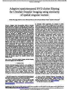
gain, α , for each controlled mode. Multiple modal controllers are run in parallel to control multiple modes. In this case the physical control force command is the sum of the individual modal control forces. Mace II STF Demonstration The MACE II system consists of the instrument structure and an electronics package containing the DSP used to implement the real-time control. The DSP software is designed to allow for guest investigators to develop and implement control algorithms in C programming language. Controllers are developed by defining several routines that are called at various stages of the real time kernel execution. To ease the development of the control systems an interface between the DSPM software and Mathworks Real Time Workshop™ (RTW) was created. RTW is a Matlab option that generates C code that duplicates the behavior of a Mathworks Simulink™ diagram. This RTW generated code is then compiled and linked with the remainder of the DSPM code to provide the executable portion of the protocol. Figure 3 is a diagram of the STF based controller used to obtain the results discussed below. b 1 (z)

1

where

fbg i

c

1

Ra n d o m Nu m b e r

1 1

a 1 (z)

1

Di scre te Fi l te r3

1 1

is the control command (generally a

1 1

force command) vector output to control the i' th

De m u x 10

!" bi g is the estimate of the modal coordinate mode, η velocity of the i' th mode generated by the STF,

v bi g

1

1

1

1

1

1

1

1

1

1

1

cusrd _ o

1

1

1

αb g

S -Fu n cti o n 1 4

Fe e d b ack G ai n 2 E t ah a t

E t ah a t 3

A number of considerations may effect the choice of forcing vector. In general the forcing vector should be chosen to project strongly on the force appropriation vector (FAV). This is desired since the resulting modal control force is the inner product of

1 1

1

De m u x

i

is the control gain and is the forcing vector. The theoretical control gain required to achieve a certain level of damping can be calculated, however, in practice it is often more effective to manually adjust control gain.

1 1

S en s ors

10 10

S e l e cto

1

Fe e d b ack 1 7 0 0 *1 1 G ai n 1

1

1 0 0 0 *1

1

6 6

1 1

1

1

1

1

Fe e d b ack G ai n

Sum 2

E t ah a t 1

1

Fe e d b ack 1 1 0 0 *1 1 G ai n 3

S e l e ctor

1

S am e

1

1

Opp

1

S en s ors

1

D is t u rb an c e

M o d a l A ctu a to rs

1

Sum 3 E t ah a t 2

S e n so rs

1

DS P M T ri p 4 S h e e t Dyn am i cs Jul y 1 4

1

4 0 0 *1

1

T o M o d a l S p a ce

Fi xe d M o d a l fi l ters

Figure 3. Block diagram of the STF based controller run on the DSPM hardware. Initial Control Results The initial goal was to develop a controller to damp out the first four structural modes of the MACE II system in the Z-direction (vertical). A MIMO configuration was set up with the six strain gauges as

6 American Institute of Aeronautics and Astronautics

Com paris on of trac e on-line vs . O ff-line 1200

is still being explored. Disturbance rejection performance was also achieved with this structural control. Figure 6 is the open and closed loop FRF from the secondary gimbal disturbance to the primary gimbal rate gyro. As can be observed, there is a significant improvement in the disturbance rejection around three of the four modes that were controlled. The two Hz mode was unaffected.

Open/Clos ed loop, S GZ-PZT1 70

60

50

40

Magnitude (dB)

inputs and the primary and secondary z-direction gimbal torques as commands. To formulate this control architecture it is necessary to estimate STF coefficients for both the sensor and the actuator arrays. The initial attempt at estimating these parameters on-line was not successful. We encountered a numerical stability problem with the RLS algorithm that was being used. The observed behavior is shown in Figure 4. This figure compares the time history of one of the STF parameters, estimated using the same data and algorithm on two different processors. Both were executed with 32-bit floating point numbers. The dark line corresponds to the behavior of the RLS algorithm on a Intel Pentium based laptop. The thin line is the behavior observed on the DSPM hardware.

30

20

10

1000

0 800

-10

600

-20

400 200

-30 0

10

20

30

40

50

60

70

Frequenc y (Hz )

0 -200 -400 4720

4740

4760

4780

4800

4820

4840

4860

4880

Figure 4. Example of numerical issue encountered on the DSPM hardware. Two lines are shown on this graph, one thick, one thin. The thick line corresponds to the parameter time history the was calculated on an IBM PC, the thin on the DSPM hardware. The momentary numerical instability is evident.

Figure 5. Demonstration of the structural control obtained. This is the FRF from the secondary gimbal z disturbance to strain gauge number one. The first four modes of the structure were controlled with velocity feedback in modal space.

Open/Closed loop, SGZ to PRGZ 10

0

-10

-20

Magnitude

This instability was not observed when the algorithm was executed in Simulink on the laptop. We are currently attempting to identify the cause of this problem.

-30

-40

-50

Control results were obtained by calculating STF coefficients offline. STF filters and force appropriation vectors for the first four structural modes were identified. The STF filters were configured to estimate the velocity corresponding to the targeted modes. These estimated modal velocities were then fed back to increase the damping of the targeted modes. The open/closed loop FRFs are shown in Figure 5. This approach is a first step towards addressing the MACE II control objectives. We focused here on controlling the resonant structural dynamics of the test article. How this relates to disturbance rejection

-60

-70

-80 0

10

20

30 40 Frequency (Hz)

50

60

70

Figure 6. Demonstration of the disturbance rejection capabilities of the STF based controller. This is the FRF from the secondary gimbal z disturbance to the primary rate gyro z. The closed loop FRF corresponds to STF based control of the first four structural modes of the system. Significant attenuation is obtained for all modes except the 1st 2Hz bending mode.

7 American Institute of Aeronautics and Astronautics

Conclusion The initial results are promising. We have achieved a significant amount of attenuation on the structural modes of the system. Controlling these structural modes significantly improves the disturbance rejection performance of the system. The numerical stability issue must be addressed. We are currently examining the assembly code generated by the TI compiler. It appears the TI compiler inappropriately truncates intermediate results, without rounding. This could be the source of our problem. Furthermore, we need to address off resonance response as well. Currently, STF techniques have been only applied to reduce resonant response. Response off resonance has not been addressed.

6.

7.

8.

9.

Shelley, S.J., Lee, K.L., Aksel, T., Aktan, A.E., "Active Control and Forced Vibration Studies on a Highway Bridge," ASCE Journal of Structural Engineering, Vol. 121, No. 9, Sept. 1995 Meirovitch, L, Baruh, H., “On the Problem of Observation Spillover in Self-Adjoint Distributed-Parameter Systems”, Journal of Optimization Theory and Application, Vol. 39, No. 2, February 1983 Widrow and S.D. Stearns, "Adaptive Signal Processing", B. , Prentice-Hall, New Jersey, 1985 Simon Haykin, "Adaptive Filter Theory", Prentice-Hall, New Jersey, 1991

Acknowledgements The authors would like to acknowledge the support received for this research under the Phase II SBIR contract awarded by the Ballistic Missile Defense Organization and managed by the AFRL, Kirtland AFB; Contract F29601-98-C-0159, Adaptive SpatioTemporal Control: A Practical Approach to Achieve Unprecedented Structural Vibration Control Performance, Robustness, and Reliability, awarded under SBIR Topic BMDO97-012.

1.

2.

3.

4.

5.

References Meirovitch, L., Baruh, H., The Implementation of Modal Filters for Control of Structures, Journal of Guidance, Control and Dynamics, Vol. 8, No. 6, November-December 1985, pp. 707-716 Shelley, S.J., Allemang, R.J., Slater, G.L., Schultze, J.F., "Active Vibration Control Utilizing an Adaptive Modal Filter Based Modal Control Method", 11'th International Modal Analysis Conference, Kissimmee, FL, Feb 1-4, 1993. Shelley, S.J., “Investigation of Discrete Modal Filters for Structural Dynamic Applications”, Doctor of Philosophy Dissertation, University of Cincinnati, 1990 Shelley, S.J., Aktan, A.E., Frederick, N., "Active Vibration Control of a 250 Foot Span Steel Truss Highway Bridge", Second IEEE Conference on Control Applications, Vancouver, B.C., September 13-16, 1993. Slater, G.L., Shelley, S.J., “Health Monitoring of Flexible Structures Using Modal Filter Concepts,” Proceedings of the 1993 North American Conference on Smart Structures and Materials, Albuquerque, New Mexico, Jan. 31 Feb. 4, 1993 8 American Institute of Aeronautics and Astronautics