The biobjective inventory routing problem – problem solution and ...

The biobjective inventory routing problem – problem solution and decision support Martin Josef Geiger and Marc Sevaux

Abstract The article presents a study on a biobjective generalization of the inventory routing problem, an important optimization problem found in logistical networks in which aspects of inventory management and vehicle routing intersect. A compact solution representation and a heuristic optimization approach are presented, and experimental investigations involving novel benchmark instances are carried out. As the investigated problem is computationally very demanding, only a small subset of solutions can be computed within reasonable time. Decision support is nevertheless obtained by means of a set of reference points, which guide the search towards the Pareto-front. Keywords: Inventory routing, computational logistics, multi-objective optimization, heuristic approaches, decision support system.

1 Introduction Many logistical activities are commonly concerned with moving required items through a graph, often referred to as a “supply chain” or “supply network”. Naturally, numerous aspects influence the way in which such processes are organized, including macro- and microeconomical conditions, the objectives of the players along the supply chain, their interrelations, and their technical abilities of communicating and thus exchanging the required information. Consequently, different implementaM.J. Geiger Helmut Schmidt University – Logistics Management Department – Hamburg, Germany. e-mail: [email protected] M. Sevaux Helmut Schmidt University – Logistics Management Department – Hamburg, Germany. Universit´e de Bretagne-Sud – Lab-STICC, Lorient, France. e-mail: marc.sevaux@ univ-ubs.fr

1

2

Martin Josef Geiger, Marc Sevaux

tions of coordination and replenishment strategies can be found in practice. While some supply chains are organized in a rather loose fashion, with sporadic interactions among the players, others consists of permanent, long-term business relations with frequent deliveries. A more recent and prominent example of how to organize the logistical activities in a supply chain is the Vendor Managed Inventory-strategy. In this approach, the vendor/ supplier takes considerable control over the inventories held at the downstream entity, i.e. the buyer/ retailer, by determining the level of inventories and the corresponding replenishment cycles/ patterns. In this sense, responsibility for adequate inventory levels is shifted upstream, while inventories as such are still held downstream. From an operations research (OR) point of view, such problems combine decision variables describing shipping quantities and dates, as well as variables determining the routing of the vehicles used for transporting the goods. The obtained models therefore lie in the intersection of two classical OR problems, namely the vehicle routing problem and inventory management problems, and have led to what is commonly referred to as inventory routing problems (IRP) [3, 18]. Inventory routing problems have drawn a considerable interest in past years. While vehicle routing and inventory management are challenging issues on their own, both aspect combined together significantly increase the difficulty of the problem at hand. Contrary to most vehicle routing problems, dynamically developing inventories require multi-period models in which deliveries are made over a certain time horizon, avoiding stockouts, if possible. On the other hand, it may be beneficial to serve customers which are close to each other together, reducing the traveled distances of the vehicles. Cost minimization in the IRP thus combines the three components of (i) costs from routing, (ii) held inventory, and (iii) stockouts. Obviously, the third component is comparably difficult to measure, and may in practice be replaced by a criterion measuring the service-level, leading to the introduction of an additional side constraint or to a multi-objective model formulation. Evaluation of solutions for the IRP nevertheless remains a difficult issue, which is why some dedicated research is going in this direction [22]. Besides these general problem characteristics, uncertainties about future demand, deliveries, production rates, etc. are often present, leading to dynamic, stochastic models [6]. Due to the difficulty of the obtained formulations, many solution approaches reintroduce some simplifying assumptions. For example in [5], the amount of goods delivered to the customers is chosen such that a pre-defined maximum inventory level is reached again, while the work of [10] concentrates on the optimization of the delivery volume only. Other simplifications address the routing, e. g. by direct deliveries to the customers [4,14,17]. Alternative approaches allow the backlogging of parts, thus treating the problem of stockouts in an particular way [1]. In the case of deterministic demand, cyclic formulations of the IRP lead to the construction of solutions with constant replenishment intervals [13, 19, 20]. Not surprisingly, solution approaches often employ (meta-) heuristics [8]. Prominent examples include Iterated Local Search [21], Variable Neighborhood Search

The biobjective inventory routing problem

3

[24], Greedy Randomized Adaptive Search [9], Memetic Algorithms [7] and decomposition approaches making used of Lagrangian relaxations [23]. Common to all ideas is that they have been successfully adopted to the particular chosen problem. Then however, and in contrast to other domains from operations research/ management science, comparably little work has been done with respect to the proposition of a common ground for experiments, such as the proposition of benchmark instances that would allow for a detailed comparison of the solution approaches. One of the few examples is found in the “Praxair”-case, an international industrial gases company facing an IRP [9]. Besides, a description of how to compute instances is given in [2]. From this perspective, the definition and publication of benchmark data allowing a future comparison appears to be a beneficial contribution. Besides, and with with respect to practical side constraints of such problems, rulebased solution approaches might provide an interesting field of research [15]. Contrary to most (meta-) heuristics, which are based on the local search paradigm, rulebased decision making approaches explicitly state why certain decision are made in particular situations. In addition to providing a solution methodology, they also contribute to the explanation of the choices made by an decision support system, thus allowing an interpretation of the system’s behavior. Moreover, human experts may directly adopt the decision making rules, an aspect that also contributes to the acceptance of such (semi-) automated optimization/ approximation approaches. This article contributes to two of the above mentioned issues of the Inventory Routing Problem. After the description of the IRP tackled in this paper in the following Sect. 2, we present a compact solution representation and a heuristic solution approach in Sect. 3. A set of benchmark instances is introduced in Sect. 4, and experimental investigations of the solution approach on the proposed data are carried out and reported. Conclusions are presented in Sect. 5.

2 Description of the investigated IRP We consider an IRP in which a given set of n customers needs to be delivered with goods from a single depot. The problem-immanent vehicle routing problem (VRP) aspects of the ones of the classical capacitated VRP. This means that we assume a unlimited number of available trucks, each of which has a limited capacity C for the delivered goods. Decision variables of the problem are on the one hand delivery quantities qit for each customer i, i = 1, . . . , n, and each period t, t = 1, . . . , T . On the other hand, a VRP must be solved for each period t of the planning horizon T , combining the delivery quantities qit into tours/ routes for the involved fleet of vehicles. We assume qit ≥ 0 ∀i, t, thus forbidding the pickup of goods at all times. Following the definition of the classical capacitated VRP, we do not permit split-deliveries, and therefore qit ≤ C ∀i, t where C is the truck capacity.

4

Martin Josef Geiger, Marc Sevaux

At each customer i, a demand dit is to be satisfied for each period t. Inventory levels Lit at the customers are limited to a maximum amount of Qi , i.e. Lit ≤ − Qi ∀i, t. An incoming material flow φ+ it and an outgoing material flow φit links the inventory levels at the customers over the time horizon: Lit+1 = Lit + φ+ it − φ− ∀i, t = 1, . . . , T − 1. it + The incoming material flow is given by φ+ it = qit iff qit ≤ Qi − Lit−1 , and φit = Qi − Lit−1 otherwise. This implies that the maximum inventory levels are never exceeded, independent from the choice of the shipping quantities qit . On the other hand, delivery quantities qit with qit > Qi −Lit−1 can be excluded when solving the problem. Obviously, as all inventory levels Lit ≥ 0, any delivery quantity qit > Qi will not play a role also. + − The outgoing material flow assumes φ− it = dit iff dit ≤ Lit−1 + φit , and φit = + Lit−1 + φit otherwise. The latter case is also referred to as a stockout-situation, and the stockout-level can be computed as dit − Lit−1 − qit . As we however assume dit to be known in advance, we can easily avoid such situations by shipping enough goods in advance or just in time. Two objective functions are considered, leading to a biobjective formulation. First, we minimize the total inventory as given in expression (1). Besides, the minimization of the total distances traveled by the vehicles for shipping the quantities in each period are of interest. While the solution of this second objective as such presents an N P-hard problem, we denote this second objective with expression (2).

min

n X T X

Lit

(1)

i=1 t=1

min

T X

VRPt (q1t , . . . , qnt )

(2)

t=1

The two objectives are clearly in conflict to each other. While large shipping quantities allow for a minimization of the routes, small quantities lead to low inventory levels over time. In between, we can expect numerous compromise solutions with intermediate values. Without any additional information or artificial assumptions about the tradeoff between the two functions, no sensible aggregation into an overall evaluation is possible. Consequently the solution of the problem at hand lies in the identification of all optimal solutions in the sense of Pareto-optimality, which constitute the Pareto-set P . Treating the IRP as a biobjective optimization problem has several advantages. First, no cost functions need to be found for the aggregation of inventory levels and routing distance. This is particularly important as some components of such underlying cost functions might vary over time, with fuel prices as a prominent example. Besides, eliciting sensible statements about tradeoffs between objectives from a decision maker can be a complicated and time consuming process. Second, it allows the analysis of the problem on a more tactical planning level. In such a

The biobjective inventory routing problem

5

setting, the effect of a reduced routing on inventory levels can be studied. This might be especially interesting for companies who want to investigate the possibilities and consequences of reducing emissions of logistical activities, such as CO2 , over a longer time horizon.

3 Solution representation and heuristic search for the IRP The solution approach of this article is based on the decomposition of the problem into two phases. (i) First, quantity decisions of when and how much to ship to each customer are made. This is done such that only customers running out of stock are served, i.e. we set qit > 0 iff dit > Lit−1 ∀i, t. (ii) Second, the resulting capacitated VRPs are solved for each period t by means of an appropriate solution approach. Solving the IRP in this sequential manner has several advantages. Most importantly, we are able to introduce a compact encoding for the first phase, which allows an intuitive illustration of how the results of the procedure are obtained. We believe this to be an important aspect especially for decision makers from the industry. Besides, searching the encoding is rather easy by means of local search/ metaheuristics.

3.1 Solution encoding Alternatives are encoded by a n-dimensional vector π = (π1 , . . . , πn ) of integers. Each element πi of the vector corresponds to a particular customer i, and encodes for how many periods the customer is served in a row (covered). In the following, we refer to these values πi as a customer delivery ‘frequency’. Precisely, if dit > Lit−1 , then qit may be computed as given in expression (3). (t−1+π ) Xi qit = min dil − Lit−1 , Qi − Lit−1 , C (3) l=t

A day-to-day delivery policy is obtained for values of πi = 1. On the other hand, large values πi ship up to the maximum of the customer/ vehicle capacity, and intermediate values lead to compromise quantities in between the two extremes. On the basis of the delivery quantities, and as mentioned above, VRPs are obtained for each period which do not differ from what is known in the scientific literature.

6

Martin Josef Geiger, Marc Sevaux

3.2 Heuristic search Throughout the optimization runs, an archive Pb of nondominated solutions is kept that presents a heuristic approximation to the true Pareto set P . By means of local search, and starting from some initial alternatives, we then aim to get closer to P , updating Pb such that dominated solutions are removed, and newly discovered nondominated ones are added. In theory, any local search strategy that modifies the frequency values of vector π might be used for finding better solutions. Clearly, values πi < 1 are not possible, and exceptional large values do not make sense either due to the upper bounds on the delivery quantities as given in expression (3).

Construction procedure First, we generate solutions for which the delivery frequency assumes identical values for all customers, starting with 1 and increasing the frequency in steps of 1, up to the point where the alternative cannot be added to Pb any more. Then, we construct alternatives for which the frequency values are randomly drawn between two values: j and j + 1, thus mixing the frequency values of the first phase and therefore computing some solutions in between the ones with purely identical frequencies. The so obtained values of π are then used to determine the delivery quantities as described above. The vehicle routing problems are then solved using two alternative algorithms. On the one hand, a classical savings heuristic [12] is employed, which allows for a comparable fast construction of the required routes/ tours. On the other hand, the more advanced record-to-record travel algorithm [16] is used. Having two alternative approaches is particularly interesting with respect to the practical use of our system. While the first algorithm will allow for a fast estimation of the routing costs, improved results are possible by means of the second approach, however at the cost of more time-consuming computations.

Improvement procedure The improvement procedure put forward in this article is based on modifying the values within π, and re-solving the subsequently modified VRPs using the algorithms mentioned above. For any element of Pb , we compute the set of neighboring solutions by modifying the values πi by ±1 while avoiding values of πi < 1. The maximum number of neighboring solutions therefore is 2n. Search for improved solution naturally terminates in case of not being able to improve any element of Pb. In this sense, the approach implements the concept of a multi-point hillclimber for Pareto-optimization. Contrary to searching all elements of Pb, a representative smaller subset of Pb can be taken for the improvement procedure. This reduces the computational effort to

The biobjective inventory routing problem

7

a considerable extent. One possibility is to assume a set of reference points, and to select the elements in Pb that minimize the distance to these reference points. As a general guideline, the reference points should be chosen such that the solutions at the extreme ends of the two objective functions (1) and (2) are present in the subset. A favorable implementation of the distance function lies in the use of the weighted Chebyshef distance metric, as it allows for a selection of convex-dominated alternatives and thus provides some theoretical advantages over other approaches.

4 Experimental investigation 4.1 Proposition of benchmark data Using the geographical information of the 14 benchmark instances given in chapter 11 of [11], new data sets for inventory routing have been proposed. While the classical VRP commonly lacks multiple-period demand data, we filled this gap by proposing three demand scenarios, each of which contains a total of T = 240 demand periods for all customers. Scenario a: The average demand of each customer is constant over time. Actual (integer) demand values for each period however are drawn from an interval of ±25% around this average. Scenario b: We assume an increasing average demand, doubling from the initial value at t = 1 to t = 240. Again, the actual demand is drawn from an interval of ±25% around this average. Scenario c: In this scenario, the average demand doubles from t = 1 to t = 120, and goes back to its initial value in t = 240, following the shape of a sinus curve. Identical to the above presented cases a deviation of ±25% around these values is allowed. The resulting set of 42 benchmark instances have been made available to the scientific community under http://logistik.hsu-hh.de/IRP.

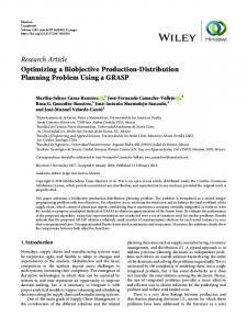
4.2 Implementation of a decision support system A test program has been developed and is used to test new and innovative strategies. Fig. 1 shows a typical screen shot of our solver. The upper part on the left gives the name of the instance and the vehicle capacity. Then below, the decision maker is able to display the different alternatives computed by the software. For the current alternative, and the current period, a text window gives the inventory level, the number of vehicle used and information on the tours. The box in the bottom left part represents the evolution of the total inventory over all periods. The

8

Martin Josef Geiger, Marc Sevaux

large window on the right presents the current alternative and period routing. Green bars are the stock level at the customer location.

Fig. 1 Screen shot of the Inventory Routing Solver.

4.3 Results Initial solutions Fig. 2 presents typical output of the frequency policies. The top left black dot is the day-to-day delivery policy, which clearly minimizes the inventory cost but has a routing cost which is important. Black dot on the bottom right represents the other alternative which apply the up-to-order policy. A large cloud of small crosses in the center results from a totally random frequency strategy. The black dots represent the solutions when all customers are served with the same frequency. To fill the gaps, a controlled random frequency (random frequencies but between two consecutive frequency values) is used and produces the results represented by white circles. Using the work done in [16], the routing cost can be improved. Fig. 3 shows the previous approximate Pareto-front resulting from the left figure with an improved routing. With low frequencies, the routing cost can be reduced greatly.

Results of local search Running the multi-point hillclimber introduced in Sect. 3.2 on all elements of Pb turns out to be not feasible for most of the proposed benchmark instances. On the

The biobjective inventory routing problem

9 Inventory-Routing alternatives

140000 Totally random frq. Controlled random frq. Identical frq.

130000

Total routing cost

120000

110000

100000

90000

80000

70000

60000 0

100000

200000

300000 400000 500000 Total inventory cost

600000

700000

800000

Fig. 2 First approximation using identical and randomized frequencies. Inventory-Routing alternatives 140000 Improved controlled frq. Improved identical frq. Former Pareto front New Pareto front

130000

Total routing cost

120000

110000

100000

90000

80000

70000

60000 0

100000

200000

300000 400000 500000 Total inventory cost

600000

700000

800000

Fig. 3 Improvements by means of the record-to-record travel algorithm.

one hand, the computations are too time consuming: Even when only making use of the savings approach for the vehicle routing part, T = 240 periods need to be solved. On the other hand, Pb is quickly populated with several thousands of solutions, and the computational effort for checking the neighborhood of all these solutions grows too large. Fig. 4 shows the obtained set of local optima for the smallest instance, scenario a, GS-01-a.irp. While the results seem to form a line/ Pareto-front, they are, indeed, 2485 discrete alternatives.

10

Martin Josef Geiger, Marc Sevaux Inventory-Routing alternatives 140000 Initial Pop. Final Pop. 130000

Total routing cost

120000

110000

100000

90000

80000

70000

60000 0

100000

200000

300000 400000 Total inventory cost

500000

600000

700000

Fig. 4 Results for instance GS-01-a.irp. Initial population and final set of local optima after applying local search.

4.4 The decision maker point of view Of course, from a theoretical point of view, having the previous results are good, even excellent. Producing 2485 alternatives ensures us to have a better coverage of the Pareto front and hence not miss any of the good solutions. But, from the decision maker point of view, this is also a very important drawback. The decision maker would wish to choose one alternative among a few, not among too many. We have then oriented our research towards the selection of representative alternatives. This is a very complicated task and can lead to errors or bad solutions. It is the reason why this specific study is still a prospective research part and will be improve in the future.

4.4.1 The global strategy The global strategy that we have implemented is the following. Among the initial population, we select a subset of solutions that, in our opinion, are a representative subset of the alternatives at the current stage. The number of solutions in this subset is a parameter that the decision maker will be able to adjust. From this subset, we start the local search on each of the alternatives and improve the solutions. We keep in an archive all the non-dominated solutions produced during this second phase. The local search is run until no more improvements are found. With this new subset of alternatives, we start again the procedure by selecting a subset of alternatives and by again running the local search over these solutions. This methods converges rather quickly (in the number of steps) but is still time consuming. Nevertheless, it comes closer to an acceptable running time for a decision

The biobjective inventory routing problem

11

maker and moreover to a good final number of alternatives for the decision maker. This will be explained with the help of Fig. 5 in the sequel.

rbc bc

bc bc

Normalized Routing Cost

bc l bc l bc bc l bc bc bc bc

r

l

l

l

l

l

bc

rbc

Normalized Inventory Cost Fig. 5 The reference set point selection and directions of search

The subset of alternatives that we select is part of the critical step. We use the reference point technique that seems to be the most appropriate in that kind of situations. To make the technique consistent, the two objectives have been normalized. Fig. 5 depicts a typical situation. The complete set of non-dominated solutions is represented by the white boxes and the two extreme solutions (the two solutions surrounded by circles at the top left corner and the bottom right corner). The two extreme solutions plus the “ideal point” (the solution circled in the bottom left corner of the figure) having the best value in terms of routing cost and inventory cost compose the three initial reference points. Then, depending on the number of final alternatives that the decision maker wants, we split the two axes (represented by the dotted line) in equal proportions. In the case presented in Fig. 5, the two axes have been split in 5, generating four additional references points for the the vertical axe and four additional reference points for the horizontal axes. These new points are represented on the figure by the black diamond. With each of the 11 reference points, we will select in the complete solution set, the solution that minimizes the Chebyshef distance metric. This will give us at most 11 solutions that will be used in the sequel for improvement as mentioned in Sect. 3.2. The direction of search is indicated on the figure with the arrows.

4.4.2 Further experiments To see how the search evolves, the different steps for a single run over instance GS-01-a.irp are reported int Table 1. The first column are the different steps identification (step 0 stands for the initial solutions). The second column reports the

12

Martin Josef Geiger, Marc Sevaux

number cumulative number of evaluation done during the search. The third column represents the size of the subset before the local search improvement phase. And the last column reports the cumulative CPU time (in seconds) of the different steps. Steps 0 1 2 3 4 5 6 7 8 9 10 11 12 13 14 15 16 17 18 19

# evaluations 235 1233 2179 3022 3962 4799 5733 6564 7320 8149 9074 9765 10355 10944 11532 11819 12105 12390 12574 12660

Subset size 28 105 150 173 198 200 221 241 243 258 261 275 280 275 272 268 274 272 269 272

Cumulative CPU (s) 34.79 221.29 387.58 535.42 699.27 844.52 1006.00 1152.02 1276.47 1424.31 1592.00 1702.35 1795.94 1883.19 1977.23 2035.96 2094.83 2153.83 2205.63 2232.77

Table 1 Evolution of the search

We can see that at step 0, i.e. we have generated 28 solutions. Among these solutions, a maximum subset of 11 solutions are selected and improved by the local search phase producing a subset of 105 non-dominated solutions for the next step. Again, from the 105 solutions, we selected 11 representatives and improve them with the local search producing 150 solutions. At the end, after 19 steps, the set of non-dominated solutions comprises 272 solutions from which we can select only 11 to present to the decision maker. As one can see, the cumulative CPU time is still large but remain acceptable since this problem is solved in a strategic phase for the company. As mentioned before, the number of reference points selected by the decision maker is the parameter that can be adapted. It clearly influences the running time of the algorithm as shown in Table 2. # RP 3 5 11

# Steps 14 19 19

# evaluations 2885 5429 12660

Subset size 113 159 272

Table 2 Evolution of running time with the number of reference points

Cumulative CPU (s) 360.30 802.59 2232.77

The biobjective inventory routing problem

13

Another good result from the method is that the quality does not depend of the number of alternatives we are going to present to the decision maker. On the same instance GS-01-a.irp, we draw the final approximate Pareto sets obtained at the end of the search with different reference set sizes. The three solutions proposed when the reference set size is 3 (RF=3) on the figure are included in the two other sets. Other solutions of R=5 are not dominated by the solutions proposed when RF=11. We expect to obtain these results with the complete set of instances.

Inventory-Routing alternatives 140000 RP=3 RP=5 RP=11

130000

Total routing cost

120000

110000

100000

90000

80000

70000

60000 0

100000

200000

300000 400000 Total inventory cost

500000

600000

700000

Fig. 6 Comparison of the final alternatives for instance GS-01-a.irp.

Finally, it is interesting to see the evolution of the search over the different steps. The complete figure showing the total set of generated solutions during the search is not worth to display since too many solutions are close to each other making the figure overloaded. Instead, we display only the subsets of solutions that we select over the search. For the same instance GS-01-a.irp, they are represented on Fig. 7. Because the figure contains different alternatives, it is necessary to have a closer look. We decided to zoom a specific section showed in Fig. 7. The result is shown in Fig. 8. On purpose, we have drawn the different solutions with a line, showing the path followed by the search over the different steps. Again, the conclusion drawn from this figure is that the solutions generated over time are not dominated by the ones of the previous iterations (otherwise they would have been eliminated from the search). Moreover, the improvement is done on both objectives, following more or less the direction imposed by the weighted Chebyshef distance measure.

14

Martin Josef Geiger, Marc Sevaux Inventory-Routing alternatives 140000

130000

Total routing cost

120000

110000

Zooming section

100000

90000

80000

70000

60000 0

100000

200000

300000 400000 Total inventory cost

500000

600000

700000

Fig. 7 Complete display of the subsets over the search for instance GS-01-a.irp and the zooming section. Path of the search 98000 Direction

97000

Total routing cost

96000

95000

94000

93000

92000 125000

130000

135000 140000 Total inventory cost

145000

150000

Fig. 8 Path of the local search for instance GS-01-a.irp.

5 Conclusions In this paper, we have presented a practical bi-objective framework for solving the inventory routing problem. We have generated a set of new instances that are available on the internet. Preliminary experiments indicate the good general impression of the solving method and need to be confirmed by further experiments. Nevertheless, with the reference set strategy, we have been able to overcome the long computational running times, and at the same time the too numerous solutions that need to be presented to the decision maker at the end.

The biobjective inventory routing problem

15

References 1. Abdelmaguid, T.F., Dessouky, M.M., Ord´on˜ ez, F.: Heuristic approaches for the inventoryrouting problem with backlogging. Computers & Industrial Engineering 56(4), 1519–1534 (2009) 2. Archetti, C., Bertazzi, L., Laporte, G., Speranza, M.G.: A branch-and-cut algorithm for a vendor managed inventory routing problem. Transportation Science 41, 382–391 (2007) 3. Baita, F., Ukovich, W., Pesenti, R., Favaretto, D.: Dynamic routing-and-inventory problems: A review. Transportation Research-A 32(8), 585–598 (1998) 4. Barnes-Schuster, D., Bassok, Y.: Direct shipping and the dynamic single-depot/multi-retailer inventory system. European Journal of Operational Research 101, 509–518 (1997) 5. Bertazzi, L., Paletta, G., Speranza, M.G.: Deterministic order-up-to level policies in an inventory routing problem. Transportation Science 36(1), 119–132 (2002) 6. Bertazzi, L., Savelsbergh, M., Speranza, M.G.: Inventory routing. In: B. Golden, S. Raghavan, E. Wasil (eds.) The Vehicle Routing Problem: Latest Advances and New Challenges, Operations Research/Computer Science Interfaces, vol. 43, pp. 49–72. Springer Science+Business Media, LLC (2008) 7. Boudia, M., Prins, C.: A memetic algorithm with dynamic population management for an integrated production-distribution problem. European Journal of Operational Research 195(3), 703–715 (2009) 8. Campbell, A.M., Savelsbergh, M.: Efficient insertion heuristics for vehicle routing and scheduling problems. Transportation Science 38(3), 369–378 (2004) 9. Campbell, A.M., Savelsbergh, M.W.P.: A decomposition approach for the inventory-routing problem. Transportation Science 38(4), 488–502 (2004) 10. Campbell, A.M., Savelsbergh, M.W.P.: Delivery volume optimization. Transportation Science 38(2), 210–223 (2004) 11. Christofides, N., Mingozzi, A., Toth, P., Sandi, C.: Combinatorial optimization. John Wiley, Chichester (1979) 12. Clarke, G., Wright, J.W.: Scheduling of vehicles from a central depot to a number of delivery points. Operations Research 12, 568–581 (1964) 13. Day, J.M., Wright, P.D., Schoenherr, T., Venkataramanan, M., Gaudette, K.: Improving routing and scheduling decisions at a distributor of industrial glass. Omega 37, 227–237 (2009) 14. Kleywegt, A.J., Nori, V.S., Savelsbergh, M.W.P.: The stochastic inventory routing problem with direct deliveries. Transportation Science 36(1), 94–118 (2002) 15. Lee, K.K.: Fuzzy rule generation for adaptive scheduling in a dynamic manufacturing environment. Applied Soft Computing 8, 1295–1304 (2008) 16. Li, F., Golden, B., Wasil, E.: A record-to-record travel algorithm for solving the heterogeneous fleet vehicle routing problem. Computers & Operations Research 34, 2734–2742 (2007) 17. Li, J.A., Wu, Y., Lai, K.K., Liu, K.: Replenishment routing problems between a single supplier and multiple retailers with direct deliveries. European Journal of Operational Research 190, 412–420 (2008) 18. Moin, N.H., Salhi, S.: Inventory routing problems: a logistical overview. Journal of the Operational Research Society 58, 1185–1194 (2007) 19. Raa, B.: New models and algorithms for the cyclic inventory routing problem. 4OR 6 (2008) 20. Raa, B., Aghezzaf, E.H.: A practical solution approach for the cyclic inventory routing problem. European Journal of Operational Research 192, 429–441 (2009) 21. Ribeiro, R., Lourenc¸o, H.R.: Inventory-routing model, for a multi-period problem with stochastic and deterministic demand. Tech. Rep. 725, Universitat Pompeu Fabra, Barcelona, Spain (2003) 22. Song, J.H., Salvelsbergh, M.: Performance measurement for inventory routing. Transportation Science 41(1), 44–54 (2007) 23. Yu, Y., Chen, H., Chu, F.: A new model and hybrid approach for larger scale inventory routing problems. European Journal of Operational Research 189, 1022–1040 (2008)

16

Martin Josef Geiger, Marc Sevaux

24. Zhao, Q.H., Chen, S., Zang, C.X.: Model and algorithm for inventory/routing decisions in a three-echelon logistics system. European Journal of Operational Research 191, 623–635 (2008)