The Boisdale Algorithm – an Induction Method for a Subclass of Unification Grammar from Positive Data Bradford Starkie1,2, and Henning Fernau2,3 1
Telstra Research Laboratories, 770 Blackburn Rd Clayton, Melbourne Victoria, 3127, Australia
[email protected] http://www.cs.newcastle.edu.au/~bstarkie/ 2 University of Newcastle, School of Electrical Engineering and Computer Science, University Drive, NSW 2308 Callaghan, Australia 3 Theoretische Informatik, Wilhelm-Schickard-Institut für Informatik, Universität Tübingen, Sand 13, D-72076 Tübingen, Germany
[email protected] http://www-fs.informatik.uni-tuebingen.de/~fernau/
Abstract. This paper introduces a new grammatical inference algorithm called the Boisdale algorithm. This algorithm can identify a class of contextfree unification grammar in the limit from positive data only. The Boisdale algorithm infers both the syntax and the semantics of the language, where the semantics of the language can be described using arbitrarily complex data structures represented as key value pairs. The Boisdale algorithm is an alignment based learning algorithm that executes in polynomial time with respect to the length of the training data and can infer a grammar when presented with any set of sentences tagged with any data structure. This paper includes a description of the algorithm, a description of a class of language that it can identify in the limit and some experimental results.
1. Introduction If an algorithm can identify a class of language in the limit from positive data only, then it is guaranteed to learn a grammar of that class exactly at some finite time when presented with an infinite stream of example sentences generated from that language. In this respect, the ability to identify a class of language in the limit is a measure of the quality of the algorithm if the objective of the learning task is to learn a language exactly. The papers of Gold [5] and Angluin [3] are the quintessential texts on identification in the limit of languages from positive data only. A brief but up-to-date introduction to the state of the art of grammatical inference of context-free grammars can be found in de la Higuera and Oncina [4]. In Starkie [9] a new grammatical inference algorithm for inferring context-free grammars was introduced called the Left-Alignment algorithm. This algorithm has the property that it can identify a class of context-free grammar in the limit from positive data only. The Boisdale algorithm described in this paper is an extension of the left alignment algorithm that enables the semantics of the language to be learnt
in addition to the syntax of the language. To this end ,we use unification grammars that are similar to Definite Clause Grammars (DCGs) Pereira and Warren [7]; both can be viewed as attributed context-free grammars. Unification grammars can be used to both convert natural language sentences into data structures (represented as key-value pairs) and to convert data structures into natural language sentences. The algorithm can infer a grammar when presented with an arbitrary set of tagged sentences, and can do so in polynomial (update) time. We also add a very brief description of a class of grammar that can be identified in the limit using the Boisdale algorithm (so-called Boisdale grammars); Starkie and Fernau [10] contains a proof showing that all Boisdale grammars can be identified in the limit from positive data only using the Boisdale algorithm. Some experimental results will be presented including an empirical confirmation that the algorithm can infer any Boisdale grammar in the limit from positive data only. Although the Boisdale algorithm can infer any Boisdale grammar in the limit from positive data, there exist some sets of training examples for which no Boisdale grammar exists that can generate those sentences amongst others. In this instance, the Boisdale algorithm still terminates and returns a unification grammar that can generate at least the training examples. The exact characterization of the class of grammars that can be identified in the limit using the Boisdale algorithm is currently an open problem.
2. Background 2.1 Notation A unification grammar is given by a 5-tuple G =(N,Σ,Π,S,A) where N is the alphabet of non-terminal symbols; Σ is the alphabet of terminal symbols with N∩Σ= { }; S is a special non-terminal called the start symbol; A is the signature definition which is an ordered list of key-type pairs (k,t) and Π is a finite set of rewrite rules of the form r = “Ni(x1..x|A|) →Ω1(x1..x|A|) … Ω|r|(x1..x|A|)” where Ni∈N,Ω i ∈(Σ∪N). The rewrite rules of G define transformations of sequences of terms to other sequences of terms. A term is comprised of a root and a signature. The root is a symbol and the signature is an ordered list of symbols. In our definition of unification grammars, all terms in the language have the same number of elements in their signature as there are elements in the signature definition. For example, the term “City(- ?fm)” has the root “City” and the signature “(- ?fm)”. In this paper we will use the symbol ‘-’ to denote an undefined value within a signature. A signature that contains only one or more instances of the symbol “-” within parentheses is referred to as the empty signature. For instance, the term “sydney(- -)” has the root “sydney" and the empty signature “(- -)”. The notation root(X) denotes the root of X. If a term does not explicitly show a signature, then it contains the empty signature, i.e., we can write “sydney” in place of “sydney(- -)”. A term Ω is either a terminal term in which case root(Ω) ∈Σ and begins with a lower case letter, or a non-terminal term in which case root(Ω) ∈N and begins with an upper case letter. A terminal term always has the empty signature. In this paper an uppercase letter is used to represent any non-terminal symbol (e.g., A), a lowercase symbol to represent any terminal symbol (e.g., a) and a Greek
letter is used to represent a symbol that could be either terminal or non-terminal (e.g., Ω or Ψ). The notation A(x) represents a term with an unknown number of symbols in its signature and |x| denotes the length of the signature. An italic uppercase letter is used to represent a sequence of zero or more terminals or non-terminal terms (e.g., A) and an italic bold uppercase letter represents a sequence of one or more terms, either terminal or non-terminal (e.g., A). The notation |A| denotes the number of terms in A. Lowercase italic letters represent a sequence of zero or more terminal terms (e.g., a) and bold italic lowercase letters represent a sequence of one or more terminal terms (e.g., a). 2.2 Unification Grammars An example unification grammar G that is described using the notation employed in this paper is given below. Relating to the formal definition introduced above, for this grammar the non-terminal alphabet is {S,City}, the terminal alphabet is {sydney,perth,perth scotland}and the signature definition is {(fm.fm),(to,fm)}. %slots {fm fm, to fm} %start S S(?fm ?to)→S(?fm -)S(- ?to) S(?fm -)→ from City(?fm -) S(- ?to)→ to City(?to -) City(SYD -)→sydney City(PTH -)→perth City(SCT -)→perth scotland
Figure 1 An example unification grammar
The first part in this denotation is the signature definition. This states that all terms in the grammar have two parameters namely a “to” attribute and an “fm” attribute. Both of these attributes are of the same type, specifically the type “fm”. As well as defining the length of the signature (two) the signature definition enables a term signature to be converted into a key-value form. For instance, the signature (PTH SYD) can be seen as the attributes {fm=PTH, to=SYD}. The start symbol of G is the non-terminal ‘S’ and all sentences that are described by this grammar (denoted L(G)) can be generated by expanding the non-terminal S until no non-terminal terms exist in the term sequence. Non-terminals can be expanded using the rewrite rules. Symbols other than ‘-’ that appear in the signature on the left-hand side of the rule and in the signature of a symbol on the right hand side are variables. (Prefixed by ‘?’ in this paper). If a rule is well formed, then for every variable in the signature of the left hand side of a rewrite rule, there is exactly one instance of that variable contained in the signature of exactly one non-terminal on the right hand side of the rewrite rule. Similarly, for every variable in the signature of a non-terminal on the right hand side of rule, there is exactly one instance of that variable in the signature on the left hand side of the rewrite rule. For instance, the rule “S(?fm ?to)→S(?fm )S(- ?to)” contains one instance of the variable “?fm” on the left hand side and exactly one instance of “?fm” on the right hand side. Before each non-terminal is expanded, all variables in the signature on the lefthand side of the rule need to be instantiated to a constant value via a process re-
ferred to as unification. Two signatures are said to unify if there is a set of mappings σ: t → u for the variables in the signatures such that if you replace the variables with their mappings, the two signatures are identical. The notation Lσ denotes the result of applying the substitution σ to L. For instance, in the above example the signature (“melbourne” “sydney”) unifies with (?fm ?to) using the mapping σ =(?fm→“melbourne”, ?to→“sydney”). That is, (?fm ?to)σ = (“melbourne” “sydney”). In contrast, the signature (“melbourne” “sydney”) does not unify with the signature (- ?to). An important method of expanding the start symbol into a terminal sequence is the rightmost expansion (denoted ⇒rm,G) in which non-terminals are expanded right to left. For example: S(“melbourne”-)S(-“sydney”) ⇒rm,G S(“melbourne”-) to City(-“sydney”). * The notation A ⇒ B denotes that A can be expanded using zero or more single step expansions to become B. A constituent is defined as an ordered pair (A , B) where A * ⇒ B. Similarly, a string can be converted to a data structure by a process referred to as reduction (denoted ⇐), where rewrite rules are applied in reverse. One important method of reduction is the leftmost reduction (denoted L,G⇐) in which reductions are applied left to right. For example:
to melbourne L,G⇐ to City(“melbourne”-) L,G⇐ S(-“melbourne”) * Similarly, the notation B ⇐ A denotes that B can be transformed to become A via zero or more single step reductions. To formally describe a leftmost reduction we need to introduce a definition of uniquely inverted that can be applied to unification grammar. A unification grammar is uniquely inverted if there are no two rules of the form A(x)→B and C(y)→D such that root(B) = root(D). Here the function root is extended to a sequence of terms as follows: root(Ω1 Ω2 .. Ωx) = root(Ω1) root(Ω2) .. root(Ωx). Formally a leftmost reduction can be described as follows: if G is uniquely inverted and A B C L,G⇐ A D(x) C then there exists a substitution ζ and a rule D(y) → Q such that Qζ = B and D(y) ζ = D(x) and there does not exist any rule of the form E(x)→F such that for some substitution ρ, A B C = H Fρ J ⇐ H E(x)ρ J and H Fρ is a proper prefix of A B. For any uniquely inverted unification grammar, the normal form achieved from a leftmost reduction is deterministic Otto [6]. It can be seen that if B * * L⇐ N(x) then N(x) ⇒ rm,G B. To describe the Boisdale algorithm, some additional notation is required. If N(y) is a term, then val(y) denotes the unordered list of values (either constants or variables) in y other than ‘-’. Let pattern(y) be a sequence of 0’s and 1’s that denotes whether each element of the signature is either ‘-’ or not ‘-‘ respectively. Let const(y) denote the unordered list of constants in y; e.g., if y = (“melbourne” - ?action 6), then val(y) = { “melbourne”, ?action, 6 }, pattern(y)=(1011) and const(y)={ “melbourne”, 6 }. The function val can be extended to terms and term sequences as follows: val(A(x))=val(x) and val(A(x) B) = val(A(x)) ∪ val(B). The functions const can be similarly expanded to reference terms and term sequences.
2.3 The Typed Leftmost Reduction We will now introduce the concept of the typed leftmost reduction. Given a set of rewrite rules, a starting term sequence and a set of constants, a typed leftmost reduction defines a deterministic set of reductions. A typed leftmost reduction is similar to a leftmost reduction in that rewrite rules are applied in a left to right sequence with the following important distinction: the definition of a typed leftmost reduction includes a set of constants c such that a rule R can only be used if const(R) ⊆ c. This is reflected by the notation L(c),G⇐.The function typed_leftmost(I,G,c) shown in Figure 2 calculates the typed leftmost reduction B such that IL(c),G⇐*B. Function typed_leftmost(I,G,c) //I a sequence of terms,G a set of rewrite rules //c a set of constants {i=0;while(i < |I|){ shift I[i] onto stack;i++; while(∃ A(x)→ B, ∃σ such that Bσ = top |B| of stack,const(x)⊆ c){ pop |B| symbols off stack;push A(x)σ onto stack;}}
Figure 2 An algorithm for calculating a typed leftmost reduction Formally, given a target set of constants c, a uniquely inverted set of rewrite rules * G and a starting sequence I a typed leftmost reduction denoted I L(c),G⇐ B is a se* * quence of reduction steps such that if I L(c)⇐ A D C L(c) ⇐ A F(x) C L(c) ⇐ B then there exists a substitution ζ and a rule F(x)ζ → Dζ such that const(x) ⊆ c and there does not exist any rule of the form E(y)→F and a substitution σ such that A D C = H * Fσ J ⇐ H E(y)σ J L⇐ B and H Fσ is a proper prefix of A D, const(y) ⊆ c. Although the definition of a typed leftmost reduction is stated in terms of a uniquely inverted grammar, we will extend the definition to enable it to be used as part of the inference process as follows: If two rules R1 and R2 can be applied at any point in a typed leftmost reduction sequence then if |const(R1)| > |const(R2)|, the sequence is reduced by R1; otherwise, the sequence is reduced by R2. 2.4 The Working Principle of the Boisdale Algorithm It can be seen that for all unification grammars, if BL(c),G⇐*A(c) then A(c)⇒*rm,G B. The Boisdale algorithm has been designed to infer grammars where for each rule there exists at least one terminal sequence, whose typed leftmost reduction recreates a rightmost derivation in reverse, i.e., for each rule of the form A(d)→E there exists * * at least one terminal string b such that A(c) ⇒rm,G Eσ ⇒ rm,G b and bL(c),G⇐ σ E L(c),G⇐A(c). The Boisdale algorithm takes as its input a set of positive training examples each tagged with key value pairs representing the meaning of those sentences. The constituents of these sentences are then guessed by aligning sentences with common prefixes from the left. In Starkie and Fernau [10] it is proven that a class of grammar exists such that aligning sentences from the left either identifies the correct constituents of the sentence, or if it incorrectly identifies constituents then those constituents will be deleted by the time the algorithm has completed. The Boisdale algorithm is believed to be one example of a class of alignment
based learning algorithms that can identify classes of unification grammar in the limit from positive data only. A related algorithm could be constructed to infer grammars for which all sentences can be reconstructed using a typed leftmost reduction, i.e., * * ∀A(c) ⇒rm,G E ⇒ rm,G b , bL(c),G⇐ EL(c),G⇐A(c). Similarly the concept of a typed rightmost reduction can be introduced that is identical to a typed leftmost reduction with the exception that reductions occur in a right to left manner. This variant of course gives rise to another class of learnable languages.
3. The Boisdale Algorithm The Boisdale algorithm begins with a set T of positive examples of the language L(G) where each s ∈ T can include a set of key value pairs (denoted attributes(s)) that describe the semantics of s. Although this algorithm uses unstructured key value pairs to describe the semantics of sentences, arbitrarily complex data structures can be mapped into assignment functions and therefore simple key-value pairs as described in Starkie [8]. (eg date.hours= “4” date.minutes=“30”). The algorithm creates a set of constituents C and hypothesis grammar H with rule set Π. The algorithm is comprised of the following 7 steps. Step 1. (Incorporation Phase) For each sentence s ∈ T, attributes(s) =x a rewrite rule of the form S(x) → s is added to H. Step 2. (Alignment Phase) Rule 1. If there exists two sentences c x1 and c x2 with a common prefix c and with attributes y1 and y2, respectively, for which the same attribute keys are defined, i.e., pattern(y1)=pattern(y2), then a new non-terminal X1 is introduced and two rules of the form X1(y5) → x1 and X1(y6) → x2 are created. The signatures of these rules (y5 and y6) are constructed such that val(y5) = val(y1) – val(y2) and val(y6) = val(y2) – val(y1). Example: When presented with the sentences “from sydney"{fm=SYD} and "from perth" {fm=PTH}, the non-terminal X48 is constructed and the rules X48(SYD -)→sydney and X48(PTH -)→perth are added to the hypothesis grammar. Rule 2. If there exists a sentence c x7 that is a prefix of another sentence c x7 x8 with attributes y7 and y8, respectively, for which the same attribute keys are defined, i.e., pattern(y7)=pattern(y8) such that there exists at least one key value pair in y7 that is not in y8 then a new non-terminal X7 is created and two rules of the form X7(y10) → x7 and X7(y11) → x7 x8 are constructed. Example: When presented with the sentences "from perth" {fm=PTH} and "from perth scotland" {fm=SCT} the non-terminal X48 is formed and the rules “X48(PTH-) →perth” and “X48(SCT -)→perth scotland” are constructed.
At this point the right hand side all of the rewrite rules of the hypothesis grammar contain only terminals. The set of constituents C is then created by copying the hypothesis grammar H, i.e., C ={ (A(x),B) | “A(x)→B”∈H }. Continue to step 3. Step 3. (Substitution Phase) The substitution phase consists of two sub phases: normalisation and completion. In both subphases, merging of non-terminals may occur. Merging non-terminals in the Boisdale algorithm involves the relabelling of some non-terminals as well as the reordering of the signatures of non-terminals. A reordering r is an array of length l where l is the number of attributes per term in the grammar. Each element of r (denoted ri) is set to either ‘-’ or an integer k such that k < l. When a signature s is reordered using a reordering r, a signature u is created such that ui = ‘-’ if ri = ‘-’, otherwise ui = sk where k= ri. After u has been constructed s is replaced by u. We will use the notation y |-|ς z to denote that y is reordered using the reordering ς to become z. Example: The signature (- SYD) can be reordered using the reordering (1 -) to become (SYD –). When the non-terminals A and C are merged using the reordering r, all signatures attached to A are reordered using r. A well-founded linear ordering