The Box Plot: A Simple Visual Method to Interpret Data. David F. Williamson, PhD; Robert A. Parker, DSc; and Juliette S. Kendrick, MD. Exploratory data analysis ...
ACADEMIA
AND
CLINIC
The Box Plot: A Simple Visual Method to Interpret Data David F. Williamson, P h D ; Robert A. Parker, DSc; and Juliette S. Kendrick, M D
Exploratory data analysis involves the use of statistical techniques to identify patterns that may be hidden in a group of numbers. One of these techniques is the "box plot," which is used to visually summarize and compare groups of data. The box plot uses the median, the approximate quartiles, and the lowest and highest data points to convey the level, spread, and symmetry of a distribution of data values. It can also be easily refined to identify outlier data values and can be easily constructed by hand. We apply box plots to tabular data from two recently published articles to show how readers can use box plots to improve the interpretation of data in complex tables. The box plot, like other visual methods, is more than a substitute for a table: It is a tool that can improve our reasoning about quantitative information. We recommend that the box plot be used more frequently. Annals of Internal Medicine.
1989; 110:916-921.
From the Centers for Disease Control, Atlanta, Georgia; and the Vanderbilt School of Medicine, Nashville, Tennessee. For current author addresses, see end of text.
1 he reader of today's medical literature faces a body of published research articles that is increasing in volume and complexity. Editors encourage brevity and conciseness (1) as more manuscripts compete for limited space ( 2 ) . Although authors are discouraged from using excessive tabular data ( 3 ) , tables are traditionally used to summarize results in less space ( 4 ) . Instead of reading an entire article, the busy reader may focus on a few key tables. However, large and complex tables may not always help the reader interpret numeric information. Recently, the editor of a journal appealed for the greater use of visual displays in communicating quantitative information in medical literature ( 5 ) .
Box Plots Authors and readers can use a simple graphic method called the "box plot" (also called a schematic plot or box-and-whiskers plot) to rapidly summarize and interpret tabular data. The box plot is one of a diverse family of statistical techniques, called exploratory data analysis, used to visually identify patterns that may otherwise be hidden in a data set. Three useful properties of exploratory data analysis techniques are that they require few prior assumptions about the data, their statistical measures are resistant to outlying data
916
values that may inordinately influence an analysis, and they emphasize visual displays that clearly highlight important landmarks of the data. Although this methodology has been well described in statistical literature (6-9), examples of its use in medical literature are rare (10). We illustrate the box plot technique, using tabular data from two recently published studies in which we were involved. Summarizing a Complex Table Powell and colleagues (11) reviewed the relation between coronary heart disease and physical inactivity in an article containing four tables of results (Tables 5 to 8), which take up ten published pages. The authors focus on the key results from 47 studies. In our Table 1, two elements are abstracted from 41 of these studies: the relative risk and the quality of the study design (0 = poor, through 3 = best). The relative risk is the ratio of the risk for coronary heart disease for the sedentary group to the risk for the most physically active group. (Relative risks could not be calculated for 6 of the 47 studies.) A relative risk of 1 implies no association between physical inactivity and coronary heart disease. Even though this table is much simpler than the four original tables, basic questions about the relation between coronary heart disease and physical inactivity are hard to answer. Although most relative risks seem to be greater than 1, how much greater is the risk of coronary heart disease among sedentary people compared with active people? How similar are the estimates of relative risk from these individual studies? Are better designed studies more likely to show an association than poorly designed studies? Figure 1 shows box plots of the data on relative risks from Table 1, subdivided by three levels of study quality. (Because there were only two studies with a quality score of 3, these were combined into one level with studies of quality score 2.) Even without understanding the details of box plots, examination of the figure readily suggests a few conclusions. The boxes are all above the line marked no association, implying that a positive association may exist between physical inactivity and coronary heart disease. The boxes shift upward as the quality measure improves. This shift suggests that better designed studies generally find stronger associations between physical inactivity and coronary heart disease. A Comparison of Three Visual Methods To understand the use of the box plot it is important
1 June 1989 • Annals of Internal Medicine • Volume 110 • Number 11
to place it in perspective with some other visual techniques, as well as to understand the details of its construction. In Figure 2 we have summarized the entire set of 41 data values from Table 1, without the study quality factor, using three alternative visual displays. The display on the left, the histogram, is the traditional visual technique for summarizing a distribution of data values. The data are grouped into equally spaced intervals and the length of each bar is directly proportional to the number of observations falling within each interval. This histogram shows that the distribution of relative risks is roughly symmetric and that the interval with the largest number of relative risks is 1.5 to 1.9. Few of the relative risks are below 1 or above 3. An exploratory data analysis technique similar to the histogram is the stem-and-leaf, the middle display Table 1. Studies Disease*
of Physical
Activity
and Coronary
Heart
Reference Number in Powell and colleagues (11)
Relative
Riskf
Quality of Study ScoreJ
58 58 32 57 14 59 93 92 107 90 39 9,10 24,25 1,2 54 8 73 73 6,64 68 67 15,56 69 99 82 82 75 75 74 35 35 35 80 58 7 70 27 27 51 87,88 40
2.0 2.3 1.9 1.8 0.5 1.1 2.0 1.2 1.8 1.1 2.8 1.9 3.1 2.0 1.6 2.5 1.1 2.4 1.6 2.0 2.0 2.6 2.4 2.3 1.6 1.5 0.9 1.5 1.2 0.5 2.5 1.6 1.4 2.2 1.5 1.1 1.5 1.1 1.7 2.5 1.9
0 0 0 1 0 0 1 2 0 0 1 1 2 1 1 1 0 0 2 1 1 2 2 1 1 1 0 0 1 0 0 2 2 0 0 0 0 0 0 3 3
* An individual published reference may contain data from more than one study. t Represents the ratio of the risk for coronary heart disease for physically inactive compared with physically active persons. % 0 = poor, 1 = good, 2 = better, 3 = best.
Figure 1. Box plots of the distributions of relative risks for coronary heart disease for physically inactive compared with physically active men from 41 studies stratified by study quality as reported in Table 1. Quality of study score was based on poor = 0, good = 1, best = 2, 3.
of Figure 2. The dark vertical line separates the decimal portion of the relative risks on the right (the leaves) from their respective grouping intervals on the left (the stems). These intervals are identical to the grouping intervals of the histogram. The asterisk represents intervals that include decimals ranging from 0.0 to 0.4, while the raised dot represents intervals that include decimals ranging from 0.5 to 0.9. For example, the relative risk 2.2 is found next to the stem labeled 2*, while the relative risk 2.8 is found next to the stem labeled 2 •. The column of numbers to the left of the stems represents the depth of each stem. Starting from each end of the distribution and working toward the middle, the depths indicate the number of values that are found up to and including each stem. For example, the depth labeled 11 indicates that there are a total of 11 relative risks included in the two intervals 0- and 1*; three are on the first stem and eight are on the second stem. In contrast to the other depths, the middle depth is given in parentheses and represents the number of data values found only on the middle stem. In this case there are 14 relative risks on the middle stem. The stem-and-leaf allows us to see the actual data values that make up the distribution, in addition to the shape, spread, and symmetry of the distribution. These details may offer insights for further analyses; for example, in the stem-and-leaf we notice that although the middle of the distribution lies within the range of values between 1.5 and 1.9, the values that most often occur (the modes) are 1.1 and 2.0. The box plot in Figure 2 provides much of the same information as the stem-and-leaf, but provides additional visual landmarks describing the distribution of relative risks, without all the detail of the stem-and-
1 June 1989 • Annals
of Internal Medicine
• Volume 110 • N u m b e r 11
917
Table 2. Sex-Specific Body Weight*
Linear Multiple
Alcohol Use By Study
Low Patients, n
HANESII Infrequent Light Moderate Heavy BRFS Infrequent Light Moderate Heavy
Regression
Regression Coefficient
Estimates
of the Degree that Alcohol
Men, A m o u n t Smokedt Medium Regression Patients, n Coefficient
Modifies
the Effect of Smoking
on
High Patients, n
Regression Coefficient
87 246 106 42
4.6 3.9 5.5 3.7
± 1.9J§ ± 1.6§ ± 1.9§ ± 2.9
133 287 143 56
1.6 3.4 2.9 -1.1
± 1.6 ± 1.3 ± 1.6 ±2.6
84 189 146 58
2.0 1.7 0.3 1.8
± 1.8 ± 1.5 ± 1.7 ±2.6
50 319 136 167
4.2 4.4 5.1 2.3
± 3.2 ± 1.8§ ±2.1§ ± 1.9
61 348 170 183
1.6 2.2 1.6 -1.4
± 3.7 ± 2.4 ±2.2 ±2.0
50 248 134 247
3.3 1.8 2.3 -2.0
± 2.8 ±2.3 ± 2.3 ±2.3
* HANESII = Second National Health and Nutrition Examination Survey; BRFS = Behavioral Risk Factor Survey. t The regression coefficient of interaction represents the joint, nonadditive effect on body weight in kilograms of smoking and alcohol. % The standard error of the regression coefficient. § The 95% CI does not overlap zero.
leaf. (By tradition the vertical axis of the box plot is read from the lowest value at the bottom to the highest value at the top, which is opposite to the stem-andleaf.) The median relative risk is just below 2.0 (horizontal line inside the box), suggesting that the average study found that a sedentary lifestyle nearly doubles the risk for a heart attack. The middle 5 0 % of the distribution of relative risks lies between 1.4 and 2.2 (ends of the box), providing a rough estimate of the variability around the median. These three visual displays summarize the overall shape, spread, and symmetry of a distribution of numbers. The histogram is the least informative of the three; the other two provide additional information that may be useful in certain situations. The stem-andleaf shows the actual values of the individual data points, and their location relative to the middle of the distribution. The box plot provides quantitative information about key aspects of the distribution, explicitly
showing the median and the extremes, as well as the variability around the median. The visual elegance of the box plot also makes it particularly useful when comparing several distributions (12). Drawing a Box Plot In the box plot of the relative risks in Figure 2, the box represents the middle 5 0 % of the data. The horizontal line inside the box is the middle or median value of the distribution of relative risks. The upper and lower ends of the box are the hinges (the approximate upper and lower quartiles) of the distribution of relative risks. The vertical lines from the ends of the box connect the extreme data points to their respective hinges. To calculate the median: 1. Rank the data values from lowest to highest. 2. Choose the value with the middle rank. If there are n data values, the median value has rank equal to (n + l ) / 2 .
Figure 2. Three different visual displays of the distribution of relative risks for coronary heart disease for physically inactive compared with physically active men from 41 studies as shown in Table 1. The 41 data values in Table 1 ranked from lowest to highest: 0.5, 0.5, 0.9, 1.1, 1.1, 1.1, 1.1, 1.1, 1.2, 1.2, 1.4, 1.5, 1.5, 1.5, 1.5, 1.6, 1.6, 1.6, 1.6, 1.7, 1.8, 1.8, 1.9, 1.9, 1.9, 2.0, 2.0, 2.0, 2.0, 2.0, 2.2, 2.3, 2.3, 2.4, 2.4, 2.5, 2.5, 2.5, 2.6, 2.8, 3.1.
918
1 June 1989 • Annals of Internal Medicine • Volume 110 • Number 11
Table 2. (Continued) Women,, Amount Smoked Low Patients, n
High
Medium Regression Coefficient
Patients, n
Regression Coefficient
Patients, n
Regression Coefficient
184 251 45 18
1.1 -0.6 3.6 -6.2
± 2.2 ± 2.0 ± 2.8 ±7.3
153 192 43 13
1.7 -0.3 3.8 3.2
± ± ± ±
1.7 1.5 2.0 7.5
91 95 45 7
-4.4 -1.8 -2.2 -6.4
± 2.7 ±2.9 ± 3.4 ±7.2
117 442 94 67
1.8 0.2 -3.0 0.3
± ± ± ±
122 377 110 85
1.0 -0.8 -0.8 -2.2
±2.3 ± 1.4 ± 1.9 ±2.1
41 226 71 66
1.8 -0.7 -3.1 -0.4
± ± ± ±
1.8 1.5 2.2 2.2
When the rank is not a whole number, the average of the values immediately above and below this rank is taken as the median value. There are 41 data values in Figure 2, so the rank of the median is (41 + l ) / 2 = 21. Counting from either end of the distribution, the 21st value is 1.8. To calculate the hinges: Add 1 to the integer rank of the median (after removing the 1/2 if there is one) and divide by 2. The lower hinge has this rank from the bottom, and the upper hinge has this rank from the top. Again, if the ranks are not whole numbers, average the values immediately above and below the ranks. In our example the rank of the median is 21; hence the rank of the upper and lower hinges is equal to (21 + l ) / 2 = 11. That is, the lower hinge is the 11th smallest data value, 1.4, whereas the upper hinge is the 11th largest value, 2.2. To complete the box plot, connect the most extreme data points (0.5 and 3.1) to their respective hinges with a vertical line. With the use of a pocket calculator, the box plot can be made more informative by identifying the unusual data points (outliers) that may deserve re-examination and verification. To identify outliers: 1. Calculate the H-spread, the distance from the lower hinge to the upper hinge. In the data in Figure 2, this is 2.2 - 1.4 = 0.8. 2. Multiply the H-spread by 1.5 and add the product to the upper hinge. Draw a dotted line there, at 3.4. This line is the outlier cutoff. 3. Stop the vertical line, showing the distribution of the data, at the largest value less than the outlier cutoff. Mark all data points that fall outside the outlier cutoff with an asterisk, and if desired, label them. 4. Carry out steps 2 and 3 on the lower hinge, remembering to subtract instead of adding. (The outlier cutoff should be drawn at 0.2.) If we assume the data come from a normal distribution, we would then expect 9 9 . 3 % of the data to be inside the outlier cutoffs ( 9 ) . The set of numbers in Figure 2 does not contain any values that qualify as outliers. When no outliers occur, the box plot is usually drawn without showing the outlier cutoffs.
2.7 2.0 3.2 3.3
Figure 1 Re-examined How do the estimates of relative risk in Table 1 relate to study quality? In Figure 1 the three box plots show clearly that the strength of the relationship between physical inactivity and risk for coronary heart disease increases as study quality improves. The median relative risk is lowest for the poor quality studies (1.5), but for the good and best quality studies, the median relative risks are similar and larger, 2.0 and 1.9, respectively. (In the good group the median and the upper hinge values coincide.) However, more telling is that the middle 5 0 % of the best group's distribution of relative risks (the box) is shifted above that of the other two groups. In addition, this figure shows that the lower modal value of 1.1, identified in the stemand-leaf, occurs only in the poor quality studies. Among the good studies, one study has a relative risk of 2.8, which now qualifies as an outlier in this box plot. The good group is a heterogeneous one: This assessment of study quality is a summary measure incorporating three characteristics of study design. This particular outlier study is one of several in the good group that were rated fairly highly on each of the three characteristics, and if a different scheme had been used to classify study quality, this particular study may have been included in the best group. The methods of the study, however, were not unusual in any way that might suggest why its results should be exceptional. We can directly conclude from Figure 1 that, based on studies of good and best quality, physically inactive persons have twice the risk for cardiovascular disease than do physically active persons. Summarizing a Complex Multivariate Analysis Box plots can also be used to help summarize complex results from multivariate analyses. We use as an example a study that examined whether alcohol modified the effect that smoking has in lowering body weight (13). This study compared the results of two national surveys, the Second National Health and Nutrition Examination Survey ( H A N E S I I ) and the Behavioral Risk Factor Survey ( B R F S ) . Both surveys catego-
1 June 1989 • Annals ofInternal Medicine • Volume 110 • Number 11
919
Figure 3. Box plots of the sex-specific distributions of the linear regression coefficients measuring the interaction between smoking and alcohol on body weight from two national surveys as shown in Table 2. HANESII is the Second National Health and Nutrition Examination Survey and BRFS is the Behavioral Risk Factor Survey.
rized cigarette consumption as none, low, medium, or high. Alcohol consumption was categorized as none, infrequent, light, moderate, or heavy. When the smoking and alcohol variables were combined, twelve interaction terms for smoking-by-drinking (for each sex and each survey) were included in the linear regression models in which body weight (in kilograms) was the dependent variable. The referent group (intercept) in the model are those who neither smoked nor drank. Table 2 (reference 13, Table 3) shows the regression coefficients for the twelve interaction terms for men and women separately, in the two national surveys. A positive coefficient indicates that alcohol diminishes the weight-lowering effect of smoking, whereas a negative coefficient indicates that alcohol magnifies the weight-lowering effect of smoking. In linear regression, a coefficient of zero implies no association. Although five coefficients were statistically different from zero, based on the tests done we would expect two to three statistically significant findings by chance alone. Furthermore, a number of the coefficients are based on small sample sizes. Hence, one is hesitant to conclude from this table alone whether or not alcohol modifies the weight-lowering effect of smoking, and whether the modification is different for men and women. Figure 3 presents box plots of the distribution of interaction coefficients for men and women in the two surveys. The medians for the interaction coefficients in men in both surveys are positive and are nearly identical in magnitude, just over 2 kilograms. One outlier was detected which prompted us to re-examine the original computer output used to produce the published results. We found no errors. However, this single occurrence may not be remarkable. We would expect a data point not to be an outlier 9 9 . 3 % of the time, assuming the underlying distribution is normal. In the four box plots of Figure 3 there are 48 data points; hence, the probability of a single outlier by
920
1 June 1989 • Annals
of Internal Medicine
chance alone is 0.29 ( 1 - 0.993 4 8 ), or nearly 1 in 3. The box plots for men also show that virtually all of the interaction coefficients are well above zero. Thus it appears that alcohol diminishes the weight-lowering effect of smoking in men. By contrast, the box plots for women show that the median interaction coefficients in both surveys are slightly negative. However, both boxes clearly overlap the null value of zero. Although the box plots themselves are quite different in appearance—one of the surveys has a wide distribution of coefficients, and the other has a compact distribution—the overall visual impression is that alcohol does not modify the weightlowering effect of smoking in women. Taken as a whole, Figure 3 represents the four-way interaction between body weight and the variables alcohol, smoking, sex, and survey. Our interpretation of this figure is that in both surveys alcohol modifies the weight-lowering effect of smoking in men but not in women. It is important to note, however, that we are not using these box plots to make a formal statistical inference about Table 2, nor to replace this highly informative table. These box plots do not provide information about the precision of the individual estimates, which is provided in Table 2, and which is necessary for parametric statistical inference. Rather, our purpose is only to show how the box plot can be used, in conjunction with a table, to explore complex relations that may be obscured when presented in tabular form alone. (See Benjamini [14] for methods to modify the box plot to convey information about the density of the distribution at each value within the box itself. These methods could conceivably be modified to convey information about the precision of each data value.)
Box Plots on the Computer Box plots can be useful in describing patterns even in very large data sets, because the box plot smooths out the numeric details while retaining important information about the distribution. Constructing box plots by hand from large data sets would be quite challenging if computer software were not available. Box plots, and other exploratory data analysis techniques, are now available on mainframe (15, 16) and microcomputers (17). However, some exploratory data analysis techniques, such as the stem-and-leaf, are not as useful for large data sets because the visual detail can be overwhelming. (It has been argued that hand calculation should be avoided even with small data sets because of possible computational errors and misinterpretation of instructions.) There are other computational procedures for estimating individual percentiles of a distribution in box plot analysis. The documentation for one commonly used statistical package lists four different computational procedures for estimating percentiles (18). Depending on the distribution of the data set, analysts using different statistical programs could conceivably produce substantially different box plots. Traditionally, hypothesis testing has not been em-
• Volume 110 • N u m b e r 11
phasized in exploratory data analysis as it requires additional assumptions about the data. Accordingly, we have not discussed methods for hypothesis testing, although this option is available on most computer programs that use box plots. For the interested reader, methods of hypothesis testing with box plots are discussed in detail by Velleman and Hoaglin ( 8 ) . Summary We have illustrated a simple but powerful way to visually interpret the distribution of a set of numbers. We have applied this technique to two complex tables that have recently been published in medical literature. This technique, the box plot, can be quickly learned and applied. Although this presentation has focused on the potential uses of box plots by readers of the literature, we also want to emphasize that box plots can be equally useful for the authors of research articles (19). In many cases, the most effective way to analyze and communicate information about a set of numbers is to draw a picture of those numbers ( 5 ) . The box plot, like other well-designed visual displays, is more than a substitute for a table: It is a tool that can improve our reasoning about quantitative information (20). Acknowledgments: The authors thank colleagues at the Centers for Disease Control who reviewed and tested the directions for constructing box plots. Requests for Reprints: David F. Williamson, PhD, Division of Nutrition, Centers for Disease Control, Room SB45-3, A-41, Atlanta, GA 30333. Current Author Addresses: Dr. Williamson: Division of Nutrition, Centers for Disease Control, Room SB45-3, A-41, Atlanta, GA 30333. Dr. Parker: Department of Preventive Medicine, Vanderbilt School of Medicine, Nashville, TN 37232. Dr. Kendrick: Division of Reproductive Health, Centers for Disease Control, Atlanta, GA 30333.
References 1. Information for authors. Am J Clin Nutr. 1987;45:141. 2. Yankauer A. Editor's report—on decisions and authorships. Am J Public Health. 1987;77:271-3. 3. Information for authors. N Engl J Med. 1987;317:96. 4. Huth EJ. How to Write and Publish Papers in the Medical Sciences. Philadelphia: ISI Press; 1982:123-6. 5. Roberts WC. The search for the masterful figure [Editorial]. Am J Cardiol. 1987;60:633-4. 6. Tukey J W . Exploratory Data Analysis. New York: Addison Wesley; 1977:39-43. 7. Mcgill R, Tukey JW, Larsen WA. Variations of boxplots. Am Stat. 1978;2:12-6. 8. Velleman PF, Hoeglin DC. Applications, Basic, and Computing of Exploratory Data Analysis. Boston: Duxbury Press; 1981. 9. Hoeglin DC, Mosteller F, Tukey JW. Understanding Robust and Exploratory Data Analysis. New York: John Wiley and Sons; 1983:63. 10. Hebert JR, Wynder EL. Dietary fat and the risk of breast cancer (Letter). N Engl J Med. 1987;317:165-6. 11. Powell KE, Thompson PD, Caspersen CJ, Kendrick JS. Physical activity and the incidence of coronary heart disease. Annu Rev Public Health. 1987;8:253-87. 12. Velleman PF, Williamson DF. Using exploratory data analysis to monitor socio-economic data quality in developing countries. In: Wright T, ed. Statistical Methods and the Improvement of Data Quality. New York: Academic Press; 1983:177-91. 13. Williamson DF, Forman MR, Binkin NJ, Gentry EM, Remington PL, Trowbridge FL. Alcohol and body weight in United States adults. Am J Public Health. 1987;77:1324-30. 14. Benjamini Y. Opening the box of a boxplot. Am Stat. 1988;42:25762. 15. SAS Institute Inc. SUGI Supplemental Library Users Guide, Version 5 Edition. Cary, North Carolina: SAS Institute, Inc.; 1986:5314. 16. Ryan TA, Joiner BL, Ryan BF. Minitab Reference Manual, Minitab Project. University Park, Pennsylvania: Pennsylvania State University; 1981. 17. Lehman RS. Statistics on the Macintosh. BYTE Magazine. 1987;(Jul)207-14. 18. SAS Institute Inc. SAS User's Guide: Basics, Version 5 Edition: The Univariate Procedure. Cary, North Carolina: SAS Institute, Inc.; 1985:1186-7. 19. Feinstein AR. X and ipr-P: an improved summary for scientific communication. / Chronic Dis. 1987;40:283-8. 20. Tufte ER. The Visual Display of Quantitative Information. Chesire, Connecticut: Graphics Press; 1983.
1 June 1989 • Annals of Internal Medicine • Volume 110 • Number 11
921