Box Plot and Box-and-Whisker Plot www.realoptionsvaluation.com
ROV Technical Papers Series: Volume 61
The Basics of Box-Whiskers In This Issue 1. Learn the basics of a box plot or box-and-whisker plot 2. Create a visual representation of outliers 3. Run box plots in Risk Simulator’s ROV BizStats 4. Compute confidence intervals using interquartile ranges
Box plots or box-and-whisker plots graphically depict numerical data using their descriptive statistics: the smallest observation (Minimum, or some variation of interquartile range), First Quartile or 25th Percentile (Q1), Median or Second Quartile or 50th Percentile (Q2), Third Quartile (Q3), and largest observation (Maximum, or some variation of interquartile range). A box plot may also indicate which observations, if any, might be considered outliers. Box plots are nonparametric in nature in that they display the differences between samples of different variables without making any assumptions of the underlying statistical distribution of the population. The distances between the various parts of the box indicate the degree of dispersion or spread and skewness in the data, and they help identify outliers. Box plots can be drawn either horizontally or vertically. The figure below on the left shows a box plot of two variables. The figure below on the right shows the location of the descriptive statistics. Notice that the individual data points are also shown in the graph as “dots.” Data points or dots beyond the endpoints may be indicative of outliers.
A Visual Representation of Outliers “How do you visually identify outliers in your data and how
Max
dispersed is your data?”
Q3 IQR Median Q1 Min
Contact Us Real Options Valuation, Inc. 4101F Dublin Blvd., Ste. 425, Dublin, California 94568 U.S.A.
[email protected] www.realoptionsvaluation.com www.rovusa.com
In Risk Simulator’s ROV BizStats module, you can generate box plots either vertically or horizontally. Further, the default box plot will be drawn based on the following five statistics as described above: Min, Q1, Median, Q3, and Max. However, ROV BizStats allows you to override the Min and Max default selections and replace them with a multiple of the InterQuartile Range (IQR), where the IQR = Q3 – Q1. Therefore, if you run the “Box Plot (Whisker Plot)” with inputs VAR1, VAR2, to VAR(N), the N box plots with the five default statistics will be displayed. However, if you also enter the optional input of say, 1.5, then the Min will be overridden with Q1 – 1.5(IQR), and the Max will be overridden with Q1 + 1.5(IQR). Usually, looking at a probability density function (PDF) of a distribution is more intuitive than looking at a box plot. However, we can still easily compare the box plot against the theoretical PDF or histogram for a normal distribution. Using a Standard Normal distribution (Normal with Mean = 0, Standard Deviation = 1), the box plot is overlaid on the PDF in the figure below. As a rule of thumb, Median ± 1.5(IQR) is around a 95% confidence interval, and Median ± 2(IQR) is around 99% confidence (two-tailed, assuming a symmetrical Gaussian-like distribution, as illustrated using a Normal distribution).
Example Calculation The example here illustrates how to obtain the confidence interval above using a Standard Normal distribution or a Normal (0,1), where the Mean = Median, or is symmetrical with zero skew. • Run the tool Risk Simulator | Analytical Tools | Probability Charts and Tables. Enter a Mean of 0 and Standard Deviation of 1 for the Normal distribution. Enter the Percentile value 0.25 and hit Enter. This will compute the 25% or Q1 standard Z-score on the left tail of –0.67449(. Recall that = 1 for the distribution. As the Normal distribution is symmetrical, the IQR or 50% confidence interval is, hence, within Median ± 0.6745( rounded. In other words, the distance between Q1 and Q3 (the IQR) is double this amount, or 1.34898(. See the figures below for details. •
Mean ± 1.5(IQR) will therefore compute to be Median ± 2.02347(. In addition, Median ± 2(IQR) will be Median ± 2.69796(. Incidentally, Median + 2(IQR) is the same as Q3 + 1.5(IQR).
In addition, for the –2.02347( value, the CDF is 2.1512% (see figure below where the random variable X is –2.02347 and CDF is computed as 0.021512). Therefore the two-tailed confidence interval would be 100% – 2(2.1512%) = 95.7% (rounded).
© Copyright 2005-2012. All rights reserved. www.realoptionsvaluation.com
Page | 2