110
9 – Intelligent Processing
THE CASCADE NEO-FUZZY ARCHITECTURE AND ITS ONLINE LEARNING ALGORITHM Yevgeniy Bodyanskiy, Yevgen Viktorov Abstract: in the paper learning algorithm for adjusting weight coefficients of the Cascade Neo-Fuzzy Neural Network (CNFNN) in sequential mode is introduced. Concerned architecture has the similar structure with the Cascade-Correlation Learning Architecture proposed by S.E. Fahlman and C. Lebiere, but differs from it in type of artificial neurons. CNFNN consists of neo-fuzzy neurons, which can be adjusted using high-speed linear learning procedures. Proposed CNFNN is characterized by high learning rate, low size of learning sample and its operations can be described by fuzzy linguistic “if-then” rules providing “transparency” of received results, as compared with conventional neural networks. Using of online learning algorithm allows to process input data sequentially in real time mode. Keywords: artificial neural networks, constructive approach, fuzzy inference, hybrid systems, neo-fuzzy neuron, real-time processing, online learning. ACM Classification Keywords: I.2.6 Learning – Connectionism and neural nets Conference: The paper is selected from Seventh International Conference on Information Research and Applications – i.Tech 2009, Varna, Bulgaria, June-July 2009
Introduction Nowadays artificial neural networks (ANNs) are widely applied for solving a large class of problems related with the processing of information given as time-series or numerical “object-property” tables generated by nonstationary, chaotic or stochastic systems. However in real conditions data processing often must be performed simultaneously with the plant functioning and therefore weight adaptation must be executed in a sequential mode as well. So called “optimization-based networks” such as Multilayer Perceptron, Radial Basis Functions Network (RBFN), Normalized Radial Basis Functions Network (NRBFN) in most cases cannot be effective during solving mentioned above problems because of their low convergence rate, curse of dimensionality, and impossibility to learn in on-line mode. In the papers [Bodyanskiy, 2008a, Bodyanskiy, 2008b, Bodyanskiy, 2008c] we have introduced various modifications of so called cascade artificial neural networks [Fahlman, 1990; Schalkoff, 1997; Avedjan, 1999], which have variable growing architecture and differs by the type of nodes – artificial neurons. It was shown that using of neo-fuzzy neurons [Yamakawa, 1992; Uchino, 1997; Miki, 1999] as elementary structural components of the cascade networks gives such valuable advantages as high learning rate, low size of the learning sample, and possibility to describe overall artificial neural network functioning process by the fuzzy linguistic “if-then” rules, what provides transparency of received results and therefore increases the range of applications for this architecture. It should be noticed that listed advantages are common for entire class of hybrid neo-fuzzy systems [Jang, 1997]. But as it was stated above possibility to adjust synaptic weight coefficients of the network is quite attractive and even necessary in some cases technique. So at this paper an attempt of synthesis of such procedure which possesses both smooth and filtering properties is taken.
The Neo-Fuzzy Neuron Neo-fuzzy neuron is a nonlinear multi-input single-output system shown in Fig.1.
International Book Series "Information Science and Computing"
111
It realizes the following mapping: n
yˆ = ∑ f i ( xi )
(1)
i =1
where xi is the i-th input (i = 1,2,…,n), yˆ is a system output. Structural blocks of neo-fuzzy neuron are nonlinear synapses NSi which perform transformation of i-th input signal in the from
f i ( xi ) =
h
∑w
ji
μ ji ( xi ).
j =1
Each nonlinear synapse realizes the fuzzy inference IF xi IS x ji THEN THE OUTPUT IS w ji where x ji is a fuzzy set which membership function is μ ji , w ji is a singleton (synaptic weight) in consequent [Uchino, 1997]. As it can be readily seen nonlinear synapse in fact realizes Takagi-Sugeno fuzzy inference of zero order. Conventionally the membership functions μ ji ( xi ) in the antecedent are complementary triangular functions. For preliminary normalized input variables xi (usually
0 ≤ xi ≤ 1 ), they can be expressed in the form: ⎧ xi − c j −1,i , x ∈ [c j −1,i , c ji ], ⎪ ⎪ c ji − c j −1,i ⎪c ⎪ j +1,i − xi , x ∈ [c ji , c j +1,i ], μ ji ( xi ) = ⎨ ⎪ c j +1,i − c ji ⎪0 − otherwise ⎪ ⎪⎩ where
c ji
yˆ
are arbitrarily selected centers of
corresponding membership functions. Usually they are equally distributed on interval [0, 1]. This contributes to simplify the fuzzy inference process. That is, an input signal xi activates only two neighboring membership functions simultaneously and the sum of the grades of these two membership functions equals to unity (Ruspini partitioning), i.e.
Figure 1. The Neo-Fuzzy Neuron
μ ji ( xi ) + μ j +1,i ( xi ) = 1. Thus, the fuzzy inference result produced by the Center-of-Gravity defuzzification method can be given in the very simple form
f i ( xi ) = w ji μ ji ( xi ) + w j +1,i μ j +1,i ( xi ). By summing up f i ( xi ) , the output yˆ of Eq. (1) is produced.
The Cascade Neo-Fuzzy Neural Network Architecture The Cascade Neo-Fuzzy Neural Network architecture shown in Fig.2 and mapping which it realizes has the following form:
9 – Intelligent Processing
112
• neo-fuzzy neuron of the first cascade
yˆ [1] =
n
h
∑∑ w
[1] ji
μ ji ( xi ),
i =1 j =1
• neo-fuzzy neuron of the second cascade
yˆ [ 2] =
n
h
∑∑ w i =1 j =1
h
[ 2] ji
μ ji ( xi ) + ∑ w[j2,n] +1 μ j ,n+1 ( yˆ [1] ), j =1
• neo-fuzzy neuron of the third cascade
yˆ [3] =
n
h
∑∑
w[ji3] μ ji ( xi ) +
i =1 j =1
h
∑
w[j3,n] +1 μ j ,n+1 ( yˆ [1] ) +
j =1
h
∑w
[ 3] j ,n + 2
μ j ,n+ 2 ( yˆ [ 2] ),
j =1
• neo-fuzzy neuron of the m-th cascade
yˆ [ m ] =
n
h
∑∑
w[jim ] μ ji ( xi ) +
i =1 j =1
n + m −1 h
∑ ∑w
[m] jl
μ jl ( yˆ [l −n ] ).
(2)
l = n +1 j =1
⎛
Thus cascade neo-fuzzy neural network contains h⎜ n +
⎝
m −1
⎞
∑ l ⎟⎠ adjustable parameters and it is important that all l =1
of them are linearly included in the definition (2). Let
us
define
h( n + m − 1) × 1
membership
functions
vector
of
m-th
neo-fuzzy
neuron
μ [ m ] = ( μ11 ( x1 ),..., μ h1 ( x1 ), μ12 ( x2 ),..., μ h 2 ( x2 ),..., μ ji ( xi ),..., μ hn ( xn ), μ1,n+1 ( yˆ [1] ),..., μ h,n+1 ( yˆ [1] ), ,..., μ h ,n+ m−1 ( yˆ m−1 ))T and
corresponding
vector
of
synaptic
weights
w[m ] =
[ m] [ m] [m] [ m] = ( w11 , w21 ,..., wh[ m1 ] , w12 ,..., wh[ m2 ] ,..., w[jim ] ,..., whn , w1[,mn+] 1 ,..., wh[ m,n]+1 ,..., wh[ m,n]+m−1 )T which has the same
dimensionality. Then we can represent expression (2) in vector notation:
yˆ [ m ] = w[ m ]T μ [ m ] .
yˆ m −1 yˆ1 yˆ 2 yˆ 3
yˆ m
Figure 2. The Cascade Neo-Fuzzy Neural Network Architecture.
International Book Series "Information Science and Computing"
113
The Cascade Neo-Fuzzy Neural Network Sequential Learning Algorithm Learning algorithm for the cascade neo-fuzzy architecture in general form can be found in [Bodyanskiy, 2008c]. It is said there that network’s growing process (increasing quantity of cascades) continues until we obtain required precision of the solved problem’s solution, and for adjusting weight coefficients of the last n-th cascade following expressions are used:
⎛ N ⎞ w ( N ) = ⎜ ∑ μ [ m ] (k ) μ [ m ]T (k ) ⎟ ⎝ k =1 ⎠
+ N
[m]
N
∑ μ [ m ] ( k ) y ( k ) = P [ m ] ( N )∑ μ [ m ] ( k ) y ( k ) k =1
(3)
k =1
in a batch mode or
⎧ [ m] P [ m ] ( k )( y (k + 1) − w[ m ]T (k ) μ [ m ] ( k + 1)) [ m ] [m] μ (k + 1), ⎪w (k + 1) = w (k ) + 1 + μ [ m ]T (k + 1) P [ m ] (k ) μ [ m ] ( k + 1) ⎪ ⎨ [m] [ m] [ m ]T (k + 1) P [ m ] (k ) [ m ] ⎪ P [ m ] (k + 1) = P [ m ] (k ) − P (k ) μ (k + 1) μ , P ( 0) = β I ⎪ 1 + μ [ m ]T ( k + 1) P [ m ] ( k ) μ [ m ] (k + 1) ⎩ or
(
(4)
)
⎧w[ m ] (k + 1) = w[ m ] (k ) + (r [ m ] (k + 1)) −1 y (k + 1) − w[ m ]T (k ) μ [ m ] (k + 1) μ [ m ] (k + 1), ⎪ ⎨ [m] 2 [m] [m] ⎪⎩r (k + 1) = αr (k ) + μ (k + 1) ,0 ≤ α ≤ 1
(5)
in a serial mode. It should be noticed that in general case algorithms (3) and (4) are not coincident since in (3)
P
[m]
P
[m]
⎛ N ⎞ (k ) = ⎜ ∑ μ [ m ] (k ) μ [ m ]T (k ) ⎟ ⎝ k =1 ⎠
+
and in (4)
If matrix
∑
N k =1
−1
⎛ N ⎞ (k ) = ⎜⎜ μ [ m ] (k ) μ [ m ]T (k ) ⎟⎟ . ⎝ k =1 ⎠
∑
μ [ m ] (k ) μ [ m ]T (k ) is singular or ill-conditioned, algorithm (4) becomes nonoperatable. And in
case we use adjusting additions P [ m ] (0) = βI , synaptic weight coefficients estimations can be significantly inaccurate and biased. Using Greville’s theorem in pseudoinversion procedure allows to write algorithm (4) in more general form [Albert, 1972]:
(
)
w[ m ] (k + 1) = w[ m ] (k ) + γ [ m ] (k + 1) y (k + 1) − w[ m ] (k ) μ [ m ] (k + 1) μ [ m ] ( k + 1),
(6)
⎧ Q[ m ] ( k ) , if μ [ m ]T ( k + 1)Q[ m ] ( k ) μ [ m ] ( k + 1) ≥ ε ( k + 1), ⎪ [ m ]T [m] [m] ( k + 1)Q ( k ) μ ( k + 1) ⎪μ Γ[ m ] ( k + 1) = ⎨ P[ m ] ( k ) ⎪ ⎪1 + μ [ m ]T ( k + 1) P[ m ] ( k ) μ [ m ] ( k + 1) , if not , ⎩
(7)
⎧ [m] Q[m] (k )μ[m] (k + 1)μ[m]T (k + 1)Q[ m] (k ) Q ( k ) − , if μ[m]T (k + 1)Q[ m] (k )μ[ m] (k + 1) ≥ ε (k + 1), ⎪ Q[ m] (k + 1) = ⎨ μ[m]T (k + 1)Q[m] (k )μ[m] (k + 1) ⎪ [m] ⎩Q (k ), if not ,
(8)
114
9 – Intelligent Processing
(
)(
) (
)(
)
)(
)
T T [m] [m] [m] [m] [m] [m] [m] [m] ⎧ P (k)μ (k +1) Q (k)μ (k +1) + Q (k)μ (k +1) P (k)μ (k +1) [ ] m ⎪P (k) − + [m]T [m] [m] ⎪ μ (k +1)Q (k)μ (k +1) ⎪ T ⎪ 1+ μ[m]T (k +1)P[m] (k)μ[m] (k +1) [m] [m] [m] [m] Q (k)μ (k +1) P (k)μ (k +1) , ⎪+ [m]T [m] 2 P (k +1) = ⎨ μ (k +1)Q[m] (k)μ[m] (k +1) ⎪ ⎪if μ[m]T (k +1)Q[m] (k)μ[m] (k +1) ≥ ε(k +1), ⎪ [m] [m] [m]T [m] ⎪ [m] P (k)μ (k +1)μ (k +1)P (k) , if not ⎪P (k) − [m]T [m] [m] 1+ μ (k +1)P (k)μ (k +1) ⎩
(
)
(
(9)
where ε ( k + 1) - nonnegative threshold which defines degree of vectors μ [ m ] ( k + 1) multi-collinearity and designates appropriate processing method. Advantages of procedure (6)-(9) are numerical stability and possibility to perform network learning when number of observations N is lesser then number of parameters which should be estimated h( n + m − 1). In case we have deal with nonstationary data, when parameters of required solution unpredictably vary with time, algorithms with exponential reducing of information value can be used, for example gradient procedure (5). If tracking speed of gradient algorithm isn’t sufficient, second order procedures can be utilized as well, for example exponentially weighted recurrent least squares method in form [Ljung, 1987]:
(
)
[m] [ m ]T [m] ⎧ P ( k ) y ( k + 1) − w ( k ) μ ( k + 1) [m] [m] [m] ⎪ w ( k + 1) = w ( k ) + μ ( k + 1), [ m ]T [m] [m] α+μ ( k + 1) P ( k ) μ ( k + 1) ⎪ ⎨ [m] [m] [ m ]T [m] 1 ⎛ [m] P ( k ) μ ( k + 1) μ ( k + 1) P ( k ) ⎞ ⎪ [m] ⎟ , 0 < α ≤ 1. ⎪ P ( k + 1) = α ⎜ P ( k ) − [ m ]T [m] [m] α+μ ( k + 1) P ( k ) μ ( k + 1) ⎠ ⎩ ⎝
(10)
It should be noticed that usage of algorithm (10) can lead to so called covariance matrix P [ m ] (k + 1) “parameters blow-up”, i.e. exponential growth of its elements. This can be avoided using valid forgetting parameter α , which usually selected in short range 0.95 ≤ α ≤ 0.99 . Decreasing α value results in rapid matrix P[ m ]−1 ( k + 1) = ∑ lk=+11α k +1−l μ [ m ] (l ) μ [ m ]T (l )
degeneration and therefore “parameters blow-up”. Usage of pseudoinverse procedure based on Greville’s theorem in algorithm (10) gives learning procedure [Bodyanskiy, 1985, Bodyanskiy, 1996, Bodyanskiy, 1998]:
(
)
w[ m ] (k + 1) = w[ m ] (k ) + γ [ m ] (k + 1) y (k + 1) − w[ m ] (k ) μ [ m ] (k + 1) μ [ m ] ( k + 1),
(11)
[m] ⎧ Q (k ) [ m ]T [m] [m] , if μ ( k + 1)Q ( k ) μ ( k + 1) ≥ ε ( k + 1), ⎪ [ m ]T [m] [m] ( k 1) Q ( k ) ( k 1) μ + μ + ⎪ [m] Γ ( k + 1) = ⎨ [m] P (k ) ⎪ ⎪ α + μ [ m ]T ( k + 1) P[ m ] ( k ) μ [ m ] ( k + 1) , if not , ⎩
(12)
(
)(
) (
)(
)
T T [m] [m] [m] [m] [m] [m] [m] [m] ⎧ ⎛ P (k)μ (k +1) Q (k)μ (k +1) + Q (k)μ (k +1) P (k)μ (k +1) 1 ⎪ ⎜ P[m] (k) − + [m]T [m] [m] ⎪α ⎜⎜ μ (k +1)Q (k)μ (k +1) ⎪ ⎝ ⎪ ⎞ ⎪ 1+ μ[m]T (k +1)P[m] (k)μ[m] (k +1) [m] [m] T [m] [m] ⎪ Q (k)μ (k +1) P (k)μ (k +1) ⎟, P[m](k +1) = ⎨+ [m]T 2 ⎟⎟ [m] [m] ⎪ μ (k +1)Q (k)μ (k +1) ⎠ ⎪ [m]T [m] [m] ⎪if μ (k +1)Q (k)μ (k +1) ≥ ε(k +1), ⎪ [m] [m] [m]T [m] ⎪1 ⎛⎜ P[m] (k) − P (k)μ (k +1)μ (k +1)P (k) ⎞⎟, if not [m]T [m] [m] ⎪⎩α ⎝ α + μ (k +1)P (k)μ (k +1) ⎠
(
)
(
)(
)
(13)
International Book Series "Information Science and Computing"
115
(here Q m (k ), Q [ m ] (k + 1) are defined by expression (8)). Proposed procedure is stable in any value of forgetting parameter. It can be seen that procedure given by equations (8), (11)-(13) is a generalization of algorithms (4), (6)-(9), and (10).
Simulation Results In order to confirm the performance of the proposed architecture the prediction of time-series is examined. We applied the proposed algorithm which allows to perform Cascade Neo-Fuzzy Neural Network learning in sequential mode for the forecasting of a chaotic process defined by the Mackey-Glass equation [Mackey, 1977]: y ′(t ) =
0, 2t (t − τ ) − 0,1 y (t ). 1 + y10 (t − τ )
(14)
The signal defined by (14) was quantized with step 0.1. We took a fragment containing 700 points. The goal was to predict time-series value on the next step k+1 using its values on steps k-3, k-2, k-1, and k. To bring into obtained set of signal values additional nonstationarity to several intervals different positive or negative numbers were added. First 500 points were used to adjust weight coefficients of the cascade architecture in sequential mode. It means that during learning procedure artificial neural network already performed time-series prediction beginning from the first element which was fed to it. Remaining 200 points were processed by cascade architecture without adjusting its weight coefficients. For simulation modeling cascade network which consists of three cascades was synthesized. Each cascade contained single neo-fuzzy neuron with three activation functions. Overall quantity of parameters which should be determined was 45. We used α = 0.985 during weight adaptation procedure in algorithm (8), (11)-(13). For estimation of received results normalized mean square error (NRMSE) as well as mean square (MSE) error was used. Obtained results of Mackey-Glass time-series prediction are shown in Fig. 3.
Figure 3. Mackey-Glass time-series prediction: original signal – solid line; network output – dashed line; prediction error – chain line. Calculated on described dataset errors were the following: MSE = 0.008, NRMSE = 0.3. As it can be readily seen from the figure signal changed its y-coordinate center four times. At each such case temporary prediction error burst occurred. Its magnitude depended on the nonstationarity power, and it’s obviously that the more drastic changes of predicted signal take place the greater error burst is happen. But after several examples are fed to network input and synaptic weight coefficients became adjusted according to changed time-series, further prediction process flows quite well. In whole, proposed algorithm for Cascade Neo-Fuzzy Neural Network gives very close approximation and prediction quality of sufficiently nonstationary processes in online mode.
116
9 – Intelligent Processing
Conclusion The new algorithm for Cascade Neo-Fuzzy Neural Network which allows to perform synaptic weight adaptation in sequential mode is proposed. It gives opportunity to start the prediction process from the first element which was fed to network’s input irrespectively from the quantity of parameters which should be determined. Theoretical justification and experiment results confirm the efficiency of developed approach.
Acknowledgements The paper is partially financed by the project ITHEA XXI of the Institute of Information Theories and Applications FOI ITHEA and the Consortium FOI Bulgaria (www.ithea.org, www.foibg.com).
Bibliography [Bodyanskiy, 2008a] Bodyanskiy Ye., Dolotov A., Pliss I., Viktorov Ye. The cascade orthogonal neural network. Advanced Research in Artificial Intelligence. Bulgaria, Sofia: Institute of Informational Theories and Applications FOI ITHEA, 2. 2008. P. 13-20. [Bodyanskiy, 2008b] Bodyansky Ye., Viktorov Ye. Time-series prediction using cascade orthogonal neural network. Radioelectronika. Informatika. Upravlinnja. №1. 2008. P. 92-97. [Bodyanskiy, 2008c] Bodyanskiy Ye., Viktorov Ye., Pliss I. The cascade neo-fuzzy neural network and its learning algorithm. Visnyk Uzhghorods’kogho Nacional’nogho universytetu. Serija “Matematyka i informatyka”, Issue 17. 2008. P. 48-58. [Fahlman, 1990] Fahlman S.E., Lebiere C. The cascade-correlation learning architecture. In: Advances in Neural Information Processing Systems. Ed. D.S. Touretzky. San Mateo, CA: Morgan Kaufman, 1990. P. 524-532. [Schalkoff, 1997] Schalkoff R.J. Artificial Neural Networks. N.Y.: The McGraw-Hill Comp., 1997. [Avedjan, 1999] Avedjan E.D., Barkan G.V., Levin I.K. Cascade neural networks. Avtomatika i Telemekhanika, 3. 1999. P. 38-55. [Yamakawa, 1992] Yamakawa T., Uchino E., Miki T., Kusanagi H. A neo fuzzy neuron and its applications to system identification and prediction of the system behavior. Proc. of 2-nd Int.Conf. on Fuzzy Logic and Neural Networks “IIZUKA-92”. Iizuka, Japan, 1992. P. 477-483. [Uchino, 1997] Uchino E., Yamakawa T. Soft computing based signal prediction, restoration and filtering. Intelligent Hybrid Systems: Fuzzy Logic, Neural Networks and Genetic Algorithms. Ed. Da Ruan. Boston: Kluwer Academic Publisher, 1997. P. 331-349. [Miki, 1999] Miki T., Yamakawa T. Analog implementation of neo-fuzzy neuron and its on-board learning. Computational Intelligence and Applications. Ed. N. E. Mastorakis. Piraeus: WSES Press, 1999. P. 144-149. [Jang, 1997] Jang Jr. S. R., Sun C. T., Mizutani E. Neuro-Fuzzy and Soft Computing. A Computational Approach to Learning and Machine Intelligence. N.J.: Prentice Hall, 1997. 614p. [Albert, 1972] Albert A. Regression and the Moore-Penrose Pseudoinverse. New York & London, Academic Press, 1972. [Ljung, 1987] Ljung L. System Identification: Theory for the User. N.J., Englewood Cliffs, Prentice-Hall. 1987. [Bodyanskiy, 1985] Bodyanskiy Ye. V., Buryak Y. O., Sodin M. L. Adaptive algorithms of identification with finite memory. Kharkiv, ruk. dep. v UkrNIINTI 05.02.1985, №218Uk, 85 Dep. 1984. 47p. [Bodyanskiy, 1996] Bodyanskiy Ye. V., Kotlyarevskiy S. V., Achkasov A. Ye., Voronovskiy G. K. Low Order Adaptive Regulators. Kharkiv, KhGAGKh. 1996. [Bodyanskiy, 1998] Bodyanskiy Ye. V., Rudenko O. G. Adaptive Models in Technical Plants Control Systems. Kyiv, UMK VO. 1998. [Mackey, 1977] Mackey M. C., Glass L. Oscillation and chaos in physiological control systems. Science, №197. 1977. P. 238-289.
Authors' Information Yevgeniy Bodyanskiy – Professor, Dr.-Ing. habil., Professor of Artificial Intelligence Department and Scientific Head of the Control Systems Research Laboratory, Kharkiv National University of Radio Electronics, Lenina av. 14, Kharkiv, 61166, Ukraine, Tel +380577021890, e-mail:
[email protected] Yevgen Viktorov - Ph.D. Student, Kharkiv National University of Radio Electronics, Lenin Av., 14, Kharkiv, 61166, Ukraine, Tel +380681613429, e-mail:
[email protected]