Mar 30, 2011 - One trace comes from a 600-machine cluster at Facebook .... reduce data size (below). FB trace. 0. 500. 1000. 0.E+00. 1.E+13. 2.E+13. 0. 1. 2.
The Case for Evaluating MapReduce Performance Using Workload Suites
Yanpei Chen Archana Ganapathi Rean Griffith Randy H. Katz
Electrical Engineering and Computer Sciences University of California at Berkeley Technical Report No. UCB/EECS-2011-21 http://www.eecs.berkeley.edu/Pubs/TechRpts/2011/EECS-2011-21.html
March 30, 2011
Copyright © 2011, by the author(s). All rights reserved. Permission to make digital or hard copies of all or part of this work for personal or classroom use is granted without fee provided that copies are not made or distributed for profit or commercial advantage and that copies bear this notice and the full citation on the first page. To copy otherwise, to republish, to post on servers or to redistribute to lists, requires prior specific permission.
The Case for Evaluating MapReduce Performance Using Workload Suites Yanpei Chen, Archana Ganapathi, Rean Griffith, Randy Katz EECS Dept., University of California, Berkeley {ychen2, archanag, rean, randy}@eecs.berkeley.edu Abstract—MapReduce systems face enormous challenges due to increasing growth, diversity, and consolidation of the data and computation involved. Provisioning, configuring, and managing large-scale MapReduce clusters require realistic, workloadspecific performance insights that existing MapReduce benchmarks are ill-equipped to supply. In this paper, we build the case for going beyond benchmarks for MapReduce performance evaluations. We analyze and compare two production MapReduce traces to develop a vocabulary for describing MapReduce workloads. We show that existing benchmarks fail to capture rich workload characteristics observed in traces, and propose a framework to synthesize and execute representative workloads. We demonstrate that performance evaluations using realistic workloads gives cluster operator new ways to identify workload-specific resource bottlenecks, and workload-specific choice of MapReduce task schedulers. We expect that once available, workload suites would allow cluster operators to accomplish previously challenging tasks beyond what we can now imagine, thus serving as a useful tool to help design and manage MapReduce systems.
I. I NTRODUCTION MapReduce is a popular paradigm for performing parallel computations on large data. Initially developed by large Internet enterprises, MapReduce has been adopted by diverse organizations for business critical analysis, such as click stream analysis, image processing, Monte-Carlo simulations, and others [1]. Open-source platforms such as Hadoop have accelerated MapReduce adoption. While the computation paradigm is conceptually simple, the logistics of provisioning and managing a MapReduce cluster are complex. Overcoming the challenges involved requires understanding the intricacies of the anticipated workload. Better knowledge about the workload enables better cluster provisioning and management. For example, one must decide how many and what types of machines to provision for the cluster. This decision is the most difficult for a new deployment that lacks any knowledge about workload-cluster interactions, but needs to be revisited periodically as production workloads continue to evolve. Second, MapReduce configuration parameters must be fine-tuned to the specific deployment, and adjusted according to added or decommissioned resources from the cluster, as well as added or deprecated jobs in the workload. Third, one must implement an appropriate workload management mechanism, which includes but is not limited to job scheduling, admission control, and load throttling. Workload can be defined by a variety of characteristics, including computation semantics (e.g., source code), data
characteristics (e.g., computation input/output), and the realtime job arrival patterns. Existing MapReduce benchmarks, such as Gridmix [2], [3], Pigmix [4], and Hive Benchmark [5], test MapReduce clusters with a small set of “representative” computations, sized to stress the cluster with large datasets. While we agree this is the correct initial strategy for evaluating MapReduce performance, we believe recent technology trends warrant an advance beyond benchmarks in our understanding of workloads. We observe three such trends: • Job diversity: MapReduce clusters handle an increasingly diverse mix of computations and data types [1]. The optimal workload management policy for one kind of computation and data type may conflict with that for another. No single set of “representative” jobs is actually representative of the full range of MapReduce use cases. • Cluster consolidation: The economies of scale in constructing large clusters makes it desirable to consolidate many MapReduce workloads onto a single cluster [6], [7]. Cluster provisioning and management mechanisms must account for the non-linear superposition of different workloads. The benchmark approach of high-intensity, short duration measurements can no longer capture the variations in workload superposition over time. • Computation volume: The computations and data size handled by MapReduce clusters increases exponentially [8], [9] due to new use cases and the desire to perpetually archive all data. This means that small misunderstanding of workload characteristics can lead to large penalties. Given these trends, it is no longer sufficient to use benchmarks for cluster provisioning and management decisions. In this paper, we build the case for doing MapReduce performance evaluations using a collection of workloads, i.e., workload suites. To this effect, our contributions are as follows: • Compare two production MapReduce traces to both highlight the diversity of MapReduce use cases and develop a way to describe MapReduce workloads. • Examine several MapReduce benchmarks and identify their shortcomings in light of the observed trace behavior. • Describe a methodology to synthesize representative workloads by sampling MapReduce cluster traces, and then execute the synthetic workloads with low performance overhead using existing MapReduce infrastructure. • Demonstrate that using workload suites gives cluster operators new capabilities by executing a particular workload to identify workload-specific provisioning bottlenecks and
inform the choice of MapReduce schedulers. We believe MapReduce cluster operators can use the workload suites to accomplish a variety of previously challenging tasks, beyond just the two new capabilities demonstrated here. For example, operators can anticipate the workload growth in different data or computational dimensions, provision the added resources just in time, instead of over-provisioning with wasteful extra capacity. Operators can also select highlyspecific configurations optimized for different kinds of jobs within a workload, instead of having uniform configurations optimized for a “common case” that may not exist. Operators can also anticipate the impact of consolidating different workloads onto the same cluster. Using the workload description vocabulary we introduce, operators can systematically quantify the superposition of different workloads across many workload characteristics. In short, once workload suites become available, we expect cluster operators to use them to accomplish innovative tasks beyond what we can now imagine. In the rest of the paper, we build the case for using workload suites by looking at production traces (Section II) and examining why benchmarks cannot reproduce the observed behavior (Section III). We detail our proposed workload synthesis and execution framework (Section IV), demonstrate that it executes representative workloads with low overhead, and gives cluster operators new capabilities (Section V). Lastly, we discuss opportunities and challenges for future work (Section VI). A. MapReduce Overview MapReduce is a straightforward divide and conquer algorithm. The input data consists of key-value pairs. It is stored on a distributed file system in mutually exclusive but jointly exhaustive partitions. A map function is applied on the input data to produce intermediate key-value pairs. The intermediate data is then shuffled to appropriate nodes, where the reduce function aggregates the intermediate data to generate the final output key-value pairs. For more details about MapReduce, we refer the reader to [10]. II. L ESSONS FROM T WO P RODUCTION T RACES There is a chronic shortage of production traces available for MapReduce researchers. Without examining these traces, it would be impossible to evaluate various proposed MapReduce benchmarks. We have access to two production Hadoop MapReduce traces, which we analyze and compare below. One trace comes from a 600-machine cluster at Facebook (FB trace), spans 6 months from May 2009 to October 2009, and contains roughly 1 million jobs. The other trace comes from a cluster of approximately 2000 machines at Yahoo! (YH trace), covers three weeks in late February 2009 and early March 2009, and contains around 30,000 jobs. Both traces contain a list of job submission and completion times, data sizes for the input, shuffle and output stages, and the running time in task-seconds of map and reduce functions (e.g., 2 task running 10 seconds each will be 20 task-seconds). Thus, these traces offer a rare opportunity to compare two large-scale MapReduce deployments using the same trace format.
CDF
CDF
1
1
0.8
0.8
0.6
0.6
input
0.4
0.4
shuffle
0.2
0.2
output
0
0 1E+0 0
1E+3 KB 1E+6 MB 1E+9 GB 1E+12 TB FB - Data size for all jobs
1E+0 1E+3 MB 1E+6 1E+9 1E+12 0 KB GB TB YH - Data size for all jobs
CDF
CDF
1
1
0.8
0.8
0.6
0.6
0.4
0.4
0.2
0.2
0
0
10-8 1E-4 10-4 1E+0 1 1E+4 104 1E+8 108 1E-8
FB - Data ratio for all jobs
output/input shuffle/input output/shuffle -8 10 -4 1E-8 1E-4 10
1E+0 1
4 8 1E+4 10 101E+8
YH - Data ratio for all jobs
Fig. 1. Data size at input/shuffle/output (top), and data ratio between
each stage (botttom).
We compare MapReduce data characteristics (Section II-A), job submission and data movement rates (Section II-B), and common jobs within each trace (Section II-C). The comparison helps us develop a vocabulary to capture key properties of MapReduce workloads (Section II-D). A. Data Characteristics MapReduce operates on key-value pairs at input, shuffle (intermediate), and output stages. The size of data at each of these stages provide a first-order indication of “what data the jobs run on”. Figure 1 shows the aggregate data sizes and data ratios at the input/shuffle/output stages, plotted as a cumulative distribution function (CDF) of the jobs in each trace. The input, shuffle, and output data sizes range from KBs to TBs in both traces. Within the same trace, the data sizes at different MapReduce stages follow different distributions. Across the two traces, the same MapReduce stage also has different distributions. Thus, the two MapReduce systems were performing different computations on different data sets. Additionally, many jobs in the FB trace have no shuffle stage the map outputs are directly written to the Hadoop Distributed File System (HDFS). Consequently, the CDF of the shuffle data sizes has a high density at 0. The data ratios between the output/input, shuffle/input, and output/shuffle stages also span several orders of magnitude. Interestingly, there is little density around 1 for the FB trace, indicating that most jobs are data expansions (ratio >> 1 for all stages) or data compressions (ratio output), expansion (input < output), transformation extract such information. We describe each job with many (input ≈ output), and summary (input >> output), with each features (dimensions), and input the array of all jobs into k- job type in varying proportions. means. K-means finds the natural clusters of data points, i.e., jobs. We consider jobs in the same cluster as belonging to a D. To Describe a Workload single equivalence class, i.e., a single “common job”. Our comparison shows that the two traces capture different We describe each job using all 6 features available from MapReduce use cases. Thus, we need a good way to describe the cluster traces - the job’s input, shuffle, output data sizes in each workload and compare it against other workloads. bytes, its running time in seconds, and its map and reduce time We believe a good description should focus on the semantics in task-seconds. We linearly normalize all data dimensions to at the MapReduce abstraction level. This includes the data
Weekly aggregate of job counts (top) and sum of map and reduce data size (below). FB trace.
Map + Reduce data size
Number of jobs
Fig. 2.
TABLE I C LUSTER SIZES , MEDIANS , AND LABELS FOR FB ( TOP ) AND YH ( BELOW ). M AP TIME AND REDUCE TIME ARE IN TASK - SECONDS , E . G ., 2 TASKS OF 10 SECONDS EACH IS 20 TASK - SECONDS . # Jobs Input Facebook trace 1081918 21 KB 37038 381 KB 2070 10 KB 405 KB 602 180 446 KB 6035 230 GB 1.9 TB 379 159 418 GB 793 255 GB 7.6 TB 19 Yahoo trace 21981 174 MB 568 GB 838 91 206 GB 7 806 GB 4.9 TB 35 5 31 TB 1303 36 GB 5.5 TB 2
Shuffle
Output
0 0 0 0 0 8.8 GB 502 MB 2.5 TB 788 GB 51 GB
871 KB 1.9 GB 4.2 GB 447 GB 1.1 TB 491 MB 2.6 GB 45 GB 1.6 GB 104 KB
73 MB 76 GB 1.5 TB 235 GB 78 GB 937 GB 15 GB 10 TB
6 MB 3.9 GB 133 MB 10 TB 775 MB 475 MB 4.0 GB 2.5 TB
Duration
Map time
Reduce time
32 s min min min min min min min min min
20 6,079 26,321 66,657 125,662 104,338 348,942 1,076,089 384,562 4,843,452
0 0 0 0 0 66,760 76,736 974,395 338,050 853,911
Small jobs Load data, fast Load data, slow Load data, large Load data, huge Aggregate, fast Aggregate and expand Expand and aggregate Data transform Data summary
min min min min min min 1 hr 4 hrs 40 min
412 270376 983998 257567 4481926 33606055 15021 7729409
740 589385 1425941 979181 1663358 31884004 13614 8305880
Small jobs Aggregate, fast Expand and aggregate Transform and expand Data summary Data summary, large Data transform Data transform, large
21 1 hr 50 1 hr 10 5 hrs 5 15 30 1 hr 25 35 55 1 35 40 2 hrs 35 3 hrs 45 8 hrs 35
on which the jobs run, the number of jobs there are in the workload and their arrival patterns, and the computation performed by the jobs. A workload description at this level will persist despite any changes in the underlying physical hardware (e.g., CPU/memory/network), or any overlaid functionality extensions (e.g., Hive or Pig). Data on which the jobs run: The data size and data ratios at the input/shuffle/output stages give a first-order description of the data. We need to describe both the statistical distribution of data sizes, and the per-job data ratios at each stage. Statistical techniques like k-means can extract the dependencies between various data dimensions. Also, the data format should be captured. Even though our traces contain no such information, data formats help us separate workloads that have the same data sizes and ratios, but different data content. Number of jobs and their arrival patterns: The list of job submissions and submission times will give a very specific description. Given that we cannot list submission times for all jobs, we should describe submission patterns using averages, peak-to-average ratios, diurnal patterns, etc. Computation performed by the jobs: The actual code for map and reduce tasks represents the most accurate description the computation done. However, the code is often unavailable due to logistical and confidentiality reasons. We believe that a good alternative is to identify classes of common jobs in the workload, similar to our k-means analysis. Here, we identify common jobs using data characteristics, job durations, and task run times. When the code is available, it would be helpful to add some semantic description, e.g., text parsing, reversing indices, image processing, detecting statistical outliers, etc. We expect this information would be available within the organizations directly managing the MapReduce clusters. The above facilitates a qualitative description. We introduce
Label
TABLE II S UMMARY OF SHORTCOMINGS OF RECENT M AP R EDUCE BENCHMARKS , COMPARED AGAINST WORKLOAD SUITES ( RIGHT- MOST COLUMN ). Gridmix2 Diverse job types Right # of jobs for each job type Variations in job submit intensity Representative data-sizes Easy to generate scaled/anticipated workloads Easy to generate consolidated workloads Cluster & config. independent
Hive BM
Hi bench √
Pig Mix √
Gridmix3 √ √
WL suites √ √
√
√
√
√ √ √
√
√
√
√
√
a quantitative description in Section IV when we describe how to synthesize a representative workload. III. S HORTCOMINGS OF M AP R EDUCE B ENCHMARKS In this section, we discuss why existing benchmarks are insufficient for evaluating MapReduce performance. Our thesis is that existing benchmarks are not representative. They capture narrow slivers of a rich space of workload characteristics. What is needed is a framework for constructing workloads that allows us to select and combine various characteristics. Table II summarizes the strengths and weaknesses of five contemporary MapReduce benchmarks – Gridmix2, Hive Benchmark, Pigmix, Hibench and Gridmix3. Below, we discuss each in detail. None of the existing benchmarks come close to the flexibility and functionality of workload suites. Gridmix2 [2] includes stripped-down versions of “common jobs” – sorting text data and SequenceFiles, sampling from large compressed datasets, and chains of MapReduce jobs exercising the combiner. Gridmix 2 is primarily a saturation tool [3], which emphasizes stressing the framework at scale. As a
result, jobs produced from Gridmix tend towards the jobs with 100s of GBs of input, shuffle, and output data. While stress evaluations are an important aspect of evaluating MapReduce performance, the production workloads in Section II contain many jobs with KB to MB data sizes. Also, as we show later in Section V-C, running a representative workload places realistic stress on the system beyond that generated by Gridmix 2. Hive Benchmark [5] tests the performance of Hive, a data warehousing infrastructure built on top of Hadoop MapReduce. It uses datasets and queries derived from those used in [12]. These queries aim to describe “more complex analytical workloads” and focus on “apples-to-apples” comparison against parallel databases. It is not clear that the queries in the Hive Benchmark reflect actual queries performed in production Hive deployments. Even if the five queries are representative, running Hive Benchmark does not capture different mixes, interleavings, arrival intensities, data sizes, etc., that one would expect in a production deployment of Hive. HiBench [13] consists of a suite of eight Hadoop programs that include synthetic microbenchmarks and real-world applications – Sort, WordCount, TeraSort, NutchIndexing, PageRank, Bayesian Classification, K-means Clustering, and EnhancedDFSIO. These programs are presented as representing a wider diversity of applications than those used in prior MapReduce benchmarking efforts. While HiBench includes a wider variety of jobs, it still fails to capture the different job mixes and job arrival rates that one would expect in production MapReduce clusters. PigMix [4] is a set of twelve queries intended to test the latency and the scalability limits of Pig – a platform for analyzing large datasets that includes a high-level language for constructing analysis programs and the infrastructure for evaluating them. While this collection of queries may be representative of the types of queries run in Pig deployments, there is no information on representative data sizes, query mixes, query arrival rate etc. to capture the workload behavior seen in production environments. Gridmix3 [14], [3] was driven by situations where improvements measured to have dramatic gains on Gridmix2 showed ambiguous or even negative effects in production [14]. Gridmix3 replays job traces collected via Rumen [15] with the same byte and record patterns and submits them to the cluster in matching time intervals, thus producing comparable load on the I/O subsystems and preserving job inter-arrival intensities. The direct replay approach reproduces inter-arrival rates and the correct mix of job types and data sizes, but introduces other shortcomings. For example, it is challenging to change the workload to add or remove new types of jobs, or to scale the workload along one or more dimensions of interest (data sizes, arrival patterns). Further, changing the input Rumen traces is difficult, limiting the benchmark’s usefulness on clusters with configurations different from the cluster that initially generated the trace. For example, the number of tasks-perjob is preserved from the traces. Thus, evaluating the appropriate configuration of task size and task number is difficult. Misconfigurations of the original cluster would be replicated.
Similarly, it is challenging to use Gridmix3 to explore the performance impact of combining or separating workloads, e.g., through consolidating the workload from many clusters, or separating a combined workload into specialized clusters. IV. W ORKLOAD S YNTHESIS AND E XECUTION We would like to synthesize a representative workload for a particular use case and execute it to evaluate MapReduce performance for a specific configuration. For MapReduce cluster operators, this approach offers more relevant insights than those gathered from one-size-fits-all benchmarks. We describe here a mechanism to synthesize representative workloads from MapReduce traces (Section IV-B), and a mechanism to execute the synthetic workload on a target system (Section IV-C). A. Design Goals We identify two design goals: 1. The workload synthesis and execution framework should be agnostic to hardware/software/configuration choices, cluster size, specific MapReduce implementation, and the underlying file system. We may intentionally vary any of these factors to quantify the performance impact of hardware choices, software (e.g., task scheduler) optimizations, configuration differences, cluster capacity increases, MapReduce implementation choices (open source vs. proprietary), or file system choices (distributed vs. local vs. in-memory). 2. The framework should synthesize representative workloads that execute in a short duration. Such workloads lead to rapid performance evaluations, i.e., rapid design loops. It is challenging to achieve both representativeness and short duration. For example, a trace spanning several months forms a workload that is representative by definition, but practically impossible to execute in full. B. Workload Synthesis The workload synthesizer takes as input a MapReduce trace over a time period of length L, and the desired synthetic workload duration W , with W < L. The MapReduce trace is a list of jobs, with each item containing the job submit time, input data size, shuffle/input data ratio, and output/shuffle data ratio. Traces with this information allow us to synthesize a workload with representative job submission rate and patterns, as well as data size and ratio characteristics. The data ratios also serve as an approximation to the actual computation being done. The approximation is a good one for a large class of IObound MapReduce computations. The workload synthesizer divides the synthetic workload into N non-overlapping segments, each of length W/N . Each segment will be filled with a randomly sampled segment of length W/N , taken from the input trace. Each sample contains a list of jobs, and for each job the submit time, input data size, shuffle/input data ratio, and output/shuffle data ratio. We concatenate N such samples to obtain a synthetic workload of length W . The synthetic workload essentially samples the trace for a number of time segments. If W