Nonlocality in the de Broglie-Bohm Interpretation of Quantum Mechanics One of the counterintuitive features of quantum mechanics is the phenomenon of nonlocality. In simple terms, this implies that, in some circumstances, particles that have interacted at some initial time and then become spatially separated remain "entangled", such that a measurement on one particle affects the other instantaneously, no matter how large the separation of the two particles has become. The standard interpretation of quantum mechanics and the de Broglie–Bohm interpretation are both consistent with experimental evidence. But it is useful to understand nonlocality if one visualizes particle trajectories rather than collapse of the wavefunction. In the trajectory approach, a measurement of one particle could lead to an incorrect prediction of the trajectory (or "surreal trajectories") of the entangled particles. The surreal trajectory is a consequence of nonlocality in which the particles are able to influence one another instantaneously. This Demonstration considers the motion of two orthogonal one-dimensional entangled particles in a Calogero–Moser potential with constant phase shift. It shows that measurement of the initial starting position of one particle affects the trajectory of the other particle. The motion of the two particles in two-dimensional configuration space might be described by a single trajectory, in which the motion is local. The projection of the trajectory onto two-dimensional configuration space leads to a decomposition of two spatially divided motions in one-dimensional real space, in which the motion becomes entangled and where quantum entanglement becomes equivalent to quantum nonlocality. Here, the configuration space represents a projection from real space, which can simulate quantum nonlocality. If the motion is entangled, chaotic, or ergodic, motion often results. Measurement of the particle position is determined by its initial choice. Mathematically, entanglement occurs if factorizability of the wavefunction is not possible; for example, when quantum superposition produces a product state, the motion becomes entangled. This means that the motion in one coordinate direction depends also on the other coordinate directions, whether the motion is periodic or 1
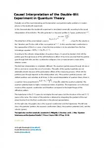
not. The component motions are independent only if the wavefunction is factorizable in configuration space. The Demonstration shows the motion in configuration space, real space, and phase space, in which the phase space consists of all possible values of position and velocity variables. The degree of entanglement is represented by the parameter a. For a=1, the wavefunction is factorizable in configuration space. The motion is periodic, and the particles behave independently of one another. The initial starting position of one particle does not affect the motion of the other particle. For a=0, the motion of the two particles becomes entangled and chaotic, depending on the constant phase shift δ. The initial starting position of a particle affects the motion of the other particle in real space. The graphic shows the trajectory in configuration space (red) and the motion of the two particles in one-dimensional real space (green and blue). If the phase space button is activated, these are shown: the x and y components of the velocity in configuration space (red), the position in the x direction, the x component of the velocity of particle 1 (blue) and the position in the y direction, and the y component of the velocity of particle 2 (green). time steps
50
3
constant phase factor
x 2
1.5
1
0 3
entanglement factor a 1. initial starting position particle 1
1.4
particle 2
1.
2
y
configuration space cs or phase space ps cs sp
1
initialize
0 10 5
t 0
Figure 1 Trajectories in the configuration space
2
Details Consider the Schrödinger equation ℏ2
𝛾𝑦
𝛾
,− 2𝑚 (𝜕𝑥,𝑥 + 𝜕𝑦,𝑦 )𝜓 + ((𝑥 2 + 𝑥𝑥2 ) + (𝑦 2 + 𝑦 2 ))𝜓 = 𝑖ℏ𝜕𝑡 𝜓
t
𝑝
with γx=γy=2, mp=1/2, ℏ=1,
x
x
, and so on. The solution involves associated
Laguerre polynomials. An entangled, un-normalized wavefunction ψ for two onedimensional particles, which cannot move along the entire x and y axes but are constrained to remain on the half x and y axes, can be expressed by a superposition state with a special parameter a: i E 1,1 t
ψ= a Θ1(x)Θ1(y)e
+ei δ Θ0(x)Θ1(y)e
i E 0,1 t
+Θ1(x)Θ0(y)e
i E 1,0 t
+ ei δ Θ0(x)Θ0(y)e
i E 0,0 t
,
where ϕk(x), ϕj(y) are eigenfunctions, and Ek,j are permuted eigenenergies of the corresponding stationary one-dimensional Schrödinger equation, with Ek,j=Ek+Ej and a,δ∈R. The eigenfunctions Θk(x), Θj(y) are given by 1
Θk,j=Θk(x)Θj(y)= x 2 αy=1/2 where
Lk
4
y
x
2
x
1
,
Lj
2 x 1
e
x2 2
Lk x x2
1
y2
2
y 1
e
y2 2
Lj
y
y2
, with αx= 1/2
4
x
1
=3/2 and
=3/2, y
y2
are associated Laguerre polynomials, and Ek,j are the quantum
numbers Ek,j= 4k+2 αx+4j+2 αy+4 with k, j ∈R. The wavefunction is taken from [1]. 𝑣𝑥 For a=1, the velocity vector v =(𝑣 ) 𝑦 in one coordinate direction does not depend on the other coordinate direction: 𝑣𝑥 (𝑥, 𝛿, 𝑡) =
(20 −
16𝑥sin(𝛿 + 4𝑡) + 4𝑡) + 4(𝑥 2 − 5)𝑥 2 + 29
8𝑥 2 )cos(𝛿
and
16𝑦sin(4𝑡) (20 − 8𝑦 2 )cos(4𝑡) + 4(𝑦 2 − 5)𝑦 2 + 29 from which the trajectory is calculated, and where x0 and y0 are the initial starting 𝑣𝑦 (𝑦, 𝑡) =
positions, which can be freely chosen for numerical integration of the velocity vector. The initial starting positions x0 (particle 1) and y0 (particle 2) can be changed by using the controls. For a=1, δ=0, and x0=y0, both components of the velocity are equal, which produces a straight line in configuration space. For the special case a=1, the trajectory becomes periodic, depending only on the constant phase shift δ in the vx term.
3
In the program, if PlotPoints, AccuracyGoal, PrecisionGoal, and MaxSteps are increased (if enabled), the results will be more accurate.
Figure 2: "Entangled" motion
References [1] M. Trott, The Mathematica GuideBook for Symbolics, New York: Springer, 2006. [2] B.-G. Englert, M. O. Scully, G. Süssman, and H. Walther, "Surrealistic Bohm Trajectories," Zeitschrift für Naturforschung A, 47(12), 1992 pp. 1175–1186. [3] "Bohmian-Mechanics.net." (Mar 16, 2016) www.bohmianmechanics.net/index.html. [4] S. Goldstein, "Bohmian Mechanics," The Stanford Encyclopedia of Philosophy. (Mar 16, 2016) plato.stanford.edu/entries/qm-bohm. [5] S. Kocsis, B. Braverman, S. Ravets, M. J. Stevens, R. P. Mirin, L. Krister Shalm, and A. M. Steinberg, "Observing the Average Trajectories of Single Photons in a Two-Slit Interferometer," Science, 332(6034), 2011 pp. 1170–1173. doi:10.1126/science.1202218. 4
[6] D. H. Mahler, L. Rozema, K. Fisher, L. Vermeyden, K. J. Resch, H. M. Wiseman, and A. Steinberg,"Experimental Nonlocal and Surreal Bohmian Trajectories," Science Advances, 2(2), 2016 pp. 1–7. doi:10.1126/science.1501466. Contributed by: Klaus von Bloh
Related Links Bohm, David Joseph (1917–1992) (ScienceWorld) Schrödinger Equation (Wolfram MathWorld) Chaos (Wolfram MathWorld) Entanglement between a Two-Level System and a Quantum Harmonic Oscillator (Wolfram Demonstrations Project) The Which-Way Experiment and the Conditional Wavefunction (Wolfram Demonstrations Project) The Causal Interpretation of a Particle in a Two-Dimensional Square Box (Wolfram Demonstrations Project) Influence of the Relative Phase in the de Broglie-Bohm Theory (Wolfram Demonstrations Project) Nodal Points in Bohmian Mechanics (Wolfram Demonstrations Project) The Caged Anharmonic Oscillator in the Causal Interpretation of Quantum Mechanics (Wolfram Demonstrations Project)
Betreff: Your submission to the Wolfram Demonstrations Project Absender: Wolfram Demonstrations Project Empfänger:
[email protected] Datum: 22. März 2016 12:30
Dear Klaus von Bloh, We are happy to inform you that your submission Nonlocality in the de Broglie-Bohm Interpretation of Quantum Mechanics to the Wolfram Demonstrations Project has been accepted for publication. Your Demonstration will now be available to all visitors to the Wolfram Demonstrations Project site.
5
The permanent URL for your Demonstration is: http://demonstrations.wolfram.com/NonlocalityInTheDeBroglieBohmInterpretationOfQua ntumMechanic/ It will be available within the next 24 hours. We encourage you to cite this Demonstration in other publications, and to send a link to the Demonstration to anyone you feel is appropriate. Please let us know if you have any questions. We look forward to receiving further Demonstrations from you in the future. Thank you for being a part of the Wolfram Demonstrations Project. Sincerely,Wolfram Demonstrations Team Wolfram Research
[email protected] http://demonstrations.wolfram.com
6