The Cellular Network as a Sensor: From Mobile

ACCEPTED FOR PUBLICATION ON IEEE TRANSACTIONS ON INTELLIGENT TRANSPORTATION SYSTEMS, 2015 (PRE-FINAL VERSION)

1

The Cellular Network as a Sensor: From Mobile Phone Data to Real-time Road Traffic Monitoring Andreas Janecek, Danilo Valerio, Karin Anna Hummel, Fabio Ricciato, Helmut Hlavacs

Abstract—Mobile cellular networks can serve as ubiquitous sensors for physical mobility. We propose a method to infer vehicle travel times on highways and to detect road congestion in real-time, based solely on anonymized signaling data collected from a mobile cellular network. Most previous studies have considered data generated from mobile devices active in calls, namely Call Detail Records (CDR), an approach that limits the number of observable devices to a small fraction of the whole population. Our approach overcomes this drawback by exploiting the whole set of signaling events generated by both idle and active devices. While idle devices contribute with a large volume of spatially coarse-grained mobility data, active devices provide finer-grained spatial accuracy for a limited subset of devices. The combined use of data from idle and active devices improves congestion detection performance in terms of coverage, accuracy, and timeliness. We apply our method to real mobile signaling data obtained from an operational network during a one-month period on a sample highway segment in the proximity of a European city, and present an extensive validation study based on groundtruth obtained from a rich set of reference datasources — road sensor data, toll data, taxi floating car data, and radio broadcast messages. Index Terms—Cellular Floating Car Data, Large Mobility Data Sets, Travel Time Estimation, Road Congestion Detection, Mobility Sensor.

I. I NTRODUCTION OLLECTING extensive information about vehicular traffic status and travel times in a timely and efficient manner is a fundamental prerequisite for intelligent transportation systems (ITSs). Traditional approaches to road traffic monitoring are prone to several technical and economical limitations [1]–[3]: systems based on roadmounted detectors or cameras suffer from high installation costs, which pose an obstacle to the full coverage of a road network, while systems based on floating car data [4]–[7] may be limited by the size and representativeness of probes, e.g., when using GPS traces from a taxi fleet or public transport vehicles. We propose an alternative approach based on the observation of the signaling traffic of a mobile cellular network. Any mobile terminal — including personal phones and tablets, but also navigation devices and on-board units (OBUs) — attached to the cellular network produces signaling messages that can be captured passively on the network side, anonymized, and then processed to derive mobility patterns. We use these messages to infer traffic status and congestion episodes on highways in real-time. Instead of a costly deployment of new sensors, we exploit the legacy cellular network as a large-scale real-time mobility sensor. The traffic information extracted with our approach can serve as a powerful input for ITS applications. The idea to extract road traffic information from cellular network data has been considered in several other studies. However, in the vast majority of previous work, traffic status reports leverage data

C

Andreas Janecek, Danilo Valerio, Helmut Hlavacs are with the Research Group Entertainment Computing, Faculty of Computer Science, University of Vienna, Austria. Danilo Valerio is also with the Telecommunication Research Center Vienna (FTW), Austria. E-mail: [email protected], [email protected], [email protected]. Karin A. Hummel is with the Communication Systems Group, Computer Engineering and Networks Lab, ETH Zurich, Switzerland, E-mail: [email protected]. Fabio Ricciato is with the Faculty of Computer and Information Science, University of Ljublijana, Slovenia, and with the Austrian Institute of Technology, Vienna, Austria: E-mail: [email protected].

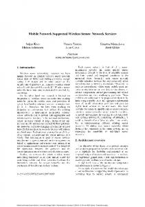
only from “active” devices, i.e., devices engaged in a voice call or data connection, based on call details records (CDR) [8]–[11]. Active devices can be tracked at cell level, i.e., with relatively high spatial accuracy, but represent only a small fraction of the device population. In our recent work [1], [12], [13], we introduced a novel approach that exploits complete signaling data captured within the cellular network infrastructure, thus extending the number of observable events. This way, also “idle” devices can be observed, which are logically attached to the cellular network but not involved in any call nor data connection. These devices can be observed at a spatial resolution of a “location area”, i.e., a spatial region consisting of multiple neighboring cells. Idle devices are the overwhelming majority of observable devices at any given time, and therefore our approach increases considerably the size of the sample set. Despite this increase in data coverage, still only a fraction of road vehicles can be observed by mobile phone data, and the question arises whether this approach provides a good estimate of the whole population of vehicles. In a first investigation, we find that this estimation is feasible. Figure 1 provides a visual comparison of the number of vehicles per hour measured by a static road sensor and the number of devices that exchanged signaling messages while traveling in the area. As can be seen, there is a strong correlation between the amount of cars on the highway and the number of mobile devices that can be tracked with our approach. Most importantly, the ratio between the two values remains stable and is almost linear. This result shows that with more complete signaling data there is no further need for dynamically compensating variations of the call habit in space and/or time, a correction task that is instead required when using CDR data. This is evident when one compares Figure 1, that includes both idle and active devices, with Figure 6 in [9, page 1434] that considers only active devices involved in calls. As noted there, the relationship between the volume of phone calls and vehicles varies with the time of day due to calling habits, e.g., there are very few calls before 8h00 despite the large number of cars during the morning rush-hour. Motivated by this preliminary finding, we develop a method to jointly process data from active and idle devices for the purpose of estimating travel times and detecting congestion episodes in real-time. We generalize the approach sketched in [13], wherein a simple algorithm based on data from idle devices was presented. We introduce algorithms to best leverage active devices in order to increase the spatial granularity of the estimation. In detail, we make the following contributions: • We present the concept of an online monitoring system for network signaling traffic that exploits the mobile cellular network as a largescale real-time sensor for mobility. In this frame, we provide a detailed description of the signaling events generated by mobile devices (Section II). • We introduce a method for estimating the expected travel time of vehicles on highway segments based solely on the signaling events observed in the network. This method features a semi-automatic approach for identifying cell pairs covering highway segments and for computing individual traversal times through the corresponding areas. The method adapts to the segment size and includes cell clustering in order to enlarge the set of traceable devices for short


Vehicles per hour

8000 Both directions (avg.) South to north North to south

6000

4000

2000

1

2

3

4

5

6

7

8

9

10

11

12

13

14

15

16

17

18

19

20

21

22

23

24

19

20

21

22

23

24

Period of day ("1" refers to 0h−1h) Phones per hour

400 Both directions (avg.) South to north North to south

300

200

100

1

2

3

4

5

6

7

8

9

10

11

12

13

14

15

16

17

18

Period of day ("1" refers to 0h−1h)

Fig. 1. Comparison of average number of vehicles per hour (upper plot) vs. average number of tracked phones per hour (lower plot) during working days (Mon-Fri) with regular traffic flow over a period of one month for one sample road section (Pearson’s correlation coefficient: 0.97). Similarly good agreement between the two profiles is found also in other road sections.

•

•

road segments (Section III). A cascaded process is presented for detecting congestion episodes from the estimated travel times across different road segments. In a first step, a congestion episode is identified based on the large set of both idle and active devices. This results in a reliable and fully automatic congestion detection. Then, the spatial accuracy is improved by reducing the observable road segment size leveraging data only from active devices (Section IV). The proposed method is demonstrated with one-month of (anonymized) signaling data from an operational cellular network, and validated against four traditional traffic monitoring datasets: road sensor data, toll data, taxi floating car data, and radio broadcast announcements (Section V). Compared to these validation data, our approach is not only more reliable in detecting congestion episodes, but also faster on average and spatially more accurate (Section VI). II. S YSTEM DESCRIPTION

We now introduce the mobile cellular network as a large-scale mobility sensor and describe the way active and idle devices are observed in the network. Further we explain how network signaling information can be used to infer physical device mobility. A. Cellular network infrastructure The infrastructure of a mobile cellular network is composed of a radio access network (RAN) and a core network (CN). The CN is divided into two distinct domains, i.e., the circuit switched (CS) and the packet switched (PS) one. Mobile devices can “attach” to the CS for voice call services, to the PS for packet data transfer, or to both domains simultaneously. Radio communication occurs between a mobile device and a fixed base station serving one or more radio cells. Cells are the smallest spatial entities in the cellular network. In general, they can be classified according to the shape and range of the coverage area. If the cell is served by an omnidirectional antenna, the coverage area can be approximated by a circle. If the cell is served by a directional antenna, the cell (also called “sector” in this case) is characterized by a beamwidth, a north-based azimuth, and a range (see Figure 2). In both cases the range of outdoor cells depends on the transmission power and the antenna design, spanning from less than hundred meters (picocells) up to several kilometers (macrocells) [14]. Depending on the radio bearer, cells can be classified as 2G (GSM/EDGE), 3G (UMTS/HSPA), or 4G

2

(LTE). A single mast usually holds several antennas, each covering a particular sector with a specific technology. At any time, each mobile device can be in active or idle state. During voice calls and data transfers, i.e., while sending and receiving IP packets, the devices are in active state. When the voice call is terminated or a timeout expires after the last data packet sent or received, the device switches to idle state and releases the radio link. Note that also “always-on” devices with permanently open data context (so called “PDP-context”, cf. [15], [16]), as typical for smartphones, remain in idle state most of the time and switch to active only upon the actual transfer of data packets. Neighboring cells are grouped into larger logical entities called Routing Areas (RAs) and Location Areas (LAs), respectively, for the PS and CS domain. One LA can contain one or more RAs, while each RA is entirely contained within one LA. In order to remain reachable, idle devices always inform the CN whenever they change LA and/or RA, i.e., they become active for a short time to communicate an LA/RA transition. Devices in active state reveal to the network also cell changes within the same LA/RA. In other words, the position of active devices is known by the network at the cell level, while the position of idle devices is known only at LA/RA level. B. Mobile phone signaling data The basis of our analysis is a sample of anonymized signaling data from the cellular network of a European country, where the network operator has about 40% market share. A passive monitoring system collects signaling messages from the links between the cellular RAN and CN covering 2G and 3G access (specifically on the IuPS, IuCS, Gb, and A interfaces [16]) and reduces the data to a stream of event-based tickets. At the time of monitoring, the network operator offered GSM, GPRS/EDGE, UMTS and HSPA access, and our dataset includes signaling messages originated by all these access technologies. The stream is delivered in near real-time to a processing machine in charge of analyzing the signaling events generated by all mobile devices registered in the network. Each ticket contains the following fields that are relevant for our study (see [13] for further details): • an anonymous identifier of the communicating device; • cell identifier, which can be mapped to the geographical cell location; • reception timestamp; • type of signaling message. The sequence of events along the visited cells allows to estimate the physical mobility of vehicles carrying devices. C. Signaling events Monitoring a mobile cellular network allows to observe a variety of signaling events generated by mobile devices in multiple cells.

Cell (sector): C Cell (sector): A azimuth: 300° azimuth: 60° beamwidth: 120° beamwidth: 120°

beamwidth= 360° Cell (sector): B azimuth: 180° beamwidth: 120°

Fig. 2. Cell with an omnidirectional antenna (left) and cells (cell sectors) A, B, and C in the case of sectoral antennas (right).


Our system is designed to take into account any signaling event that can be captured by the network monitoring system, including cell handovers, consecutive calls, SMSs, LA/RA updates (i.e., change of LA/RA), and also opening of sporadic data connections, e.g., from smartphones that periodically acquire the radio link, perform some background activity, and then release it. This results in a clear advantage of our approach compared to previous works that were limited to cell handovers of active devices, but also imposes additional challenges due to the marked heterogeneity of the observed signaling events. To illustrate the gain in terms of mobility information, we sketch in Figure 3 a sample vehicle driving along a generic highway segment. The road segment is covered by three different LAs (A, B, and C), each consisting of several cells (A1 · · · An , B1 · · · Bm , and C1 · · · Ck , respectively). The maximum amount of mobility information would be captured if a device in the vehicle is involved in a call during the entire time (row “Active terminals” in the figure). In reality, this happens very rarely. The vast majority of devices, especially on the road, are not engaged in long-lasting phone calls, i.e., they remain in “idle” state most of the time (the row “Idle terminals” shows events generated when the device remains in idle state for the whole period). Figure 3 depicts a plausible signaling pattern, which consists of LA changes/updates (“u”), phone calls (“c”), SMS messages (“s”), and data connections (“d”). In the traditional approach, cell handover events from active calls are observed (row (a)). The method proposed in [9] extends this approach by considering pairs of consecutive calls (e.g., calls c3 ,c4 in row (b)). Finally, row (c) shows what our system is able to capture by observing all different types of signaling event. We remark that obtaining the full set of (anonymized) signaling data is in general technically more complex and expensive than collecting CDR data. However, this is still feasible at reasonable marginal costs, considering that many network operators already run powerful monitoring systems in support of network operation and troubleshooting processes. The investment in the additional required monitoring infrastructure can be justified whenever a proper business model is in place to monetize the more accurate and complete mobility information that can be extracted from such data. III. T RAVEL T IME E STIMATION Road traffic may be described in terms of travel time or, alternatively, vehicle speed. Along the highway, the speed of the fastest vehicles — excluding special vehicles such as emergency vehicles — allows to capture slowed-down traffic best. Thus, we focus on the travel times experienced by the fastest vehicles. Our objective is to estimate the minimum travel times on sequences of road segments based solely on (i) the signaling exchanged between mobile terminals and the cellular network and (ii) the geographical position and antenna configuration (orientation and beamwidth) of the cellular base stations where the signaling is observed. The travel time is defined as the time required to pass through a road segment located between the boundaries of two cells exposed to signaling events, i.e., a cell pair. As the trespassing of the cell boundaries cannot be directly observed, the travel time cannot be calculated directly but must be inferred from the available signaling data. To this end, we consider the difference between the time-stamps of two signaling events observed in distinct cells within a cell pair, which we term the traversal time. In the following, we first explain how cell pairs are identified and associated to road segments. Then, we present a robust method to infer the expected travel time for selected road segments based on the set of measured traversal times between the corresponding cell pairs. Finally, we extend our approach by considering clusters of cells instead of single cells for pairing, so

3

as to include more devices into the measurements and improve the performances. A. Identification of cell pairs and cell sequences Signaling events are reported from all devices attached to a cell. In a preliminary step we identify the subset of cells serving devices that are traveling along the highway under investigation, and pair them. One option is to rely on a fully manual procedure based on visual inspection of the cell coverage map. This requires significant effort, especially if the radio network design is complex and involves multiple layers. Instead, we follow a semi-automatic procedure: in a first phase cells are selected and paired by an automatic algorithm, leaving only the final selection of pairs to a manual step. The first phase is carried out by Algorithm 1, which identifies cell pairs in proximity of the highway based on the number of traversing devices in each direction. The result is a set of ordered cell pairs (cs , ca ), where cs is the “start cell” and ca the “arrival cell”. Throughout this paper we assume that the highway is the fastest connection between cs and ca , i.e., the fastest mobile device users are all traveling on the target highway. Note that we consider ordered pairs to account for the driving direction. The methodology for estimating travel times can be applied independently to both directions. Algorithm 1 – Cell pair identification Require: Run for test period tmax ⇐ the maximum traversal time (constant value which assures that vehicles, i.e., devices, will be able to drive through this segment also during heavy congestion episodes) xmin ⇐ the minimum number of devices required P ⇐ set containing all cells in proximity of the highway for all cs ∈ P do for all ca ∈ P do if the ordered pair (cs , ca ) tracks devices traveling in the direction under investigation then For each pair (cs , ca ): count the number of mobile devices that create an event in cell cs and another event in cell ca within the time frame of tmax end if end for end for return All ordered pairs (cs , ca ) which are able to track more than xmin devices per day Out of the set produced by Algorithm 1, the final pairs associated to various highway segments are then selected based on the following (partly counteracting) criteria: 1) A cell pair should track the largest number of devices in order to guarantee reliability of the travel time estimation. This criterion tends to pick pairs consisting of LA entry cells wherein idle devices typically generate a large number of LA update events. 2) A cell pair should cover the shortest possible highway segment in order to improve spatial accuracy. This tends to include internal segments within an LA which can be observed only through active devices. The resulting final set will include at least one cell pair between LA boundaries (observed mostly but not exclusively via idle devices) plus a variable number of shorter pairs (within one LA or across two subsequent LAs) depending on the density of active devices. B. Computation of individual traversal times For every device i traversing a cell pair (cs , ca ) we compute the a,f individual traversal time ti = ta,f − ts,l is the first event i i , where ti

bu y ac

.c

tr

k e r- s o ft w a


Highway and coverage area of cells (simplified)

Active terminals

A1

LAA

A2 A3

A4

A5

A6 A7

B3 B4 A9 A 10 B1B2 A8

B5

B6

B7 B8

B9

B10

om

lic k C

.c

om

lic k C

to

bu y to

re

.

.

k e r- s o ft w a

w

w

ac

ww

ww

tr

4

B11 C1 C2

C3 …

LAC

LAB

A1 A2 A3 A4 A5 A6 A7 A8 A9 A10 B1 B2B3 B4 B5 B6 B7 B8 B9 B10B11 C1 C2 C3

Idle terminals Real-world example

u1

d1

s1

c1

c2

u2

d2

c3

c4

s2

u3

d3

(a) cell handovers (b) cell handovers and consecutive calls (c) all events

v∗ =

dsa ≤v ta,f − ts,l i i

−ti

Da

Tightest lower bound v*

dsa

cell cs Ds

T1 T2 T3

T4 T5

time

Fig. 4. Spatio-temporal representation of the traversal time calculation between two cells cs , ca at distance dsa . The linear distance along the highway (from an arbitrary reference point) is reported on the vertical axis. Each signaling message — three in cell cs and two in cell ca in this illustration — carry accurate timing information and only cell-level spatial information.

(1)

represents the tightest lower bound to the real (unknown) average speed v that can be computed from the data at hand. In other words, the generic device i must travel at least at speed v ∗ between the two cells in order to match the observed sequence of messages. By using this lower bound, we potentially underestimate the vehicle speed, but never overestimate it. This feature is key to the success of our method. In fact, as we aim to characterize the traversal time of the fastest users in order to capture slow-down effects, our approach is extremely sensitive to systematic overestimation of vehicle speed, but tolerates well a certain degree of speed underestimation. Recalling equation (1), estimating the traversal time by ta,f − ts,l i i for the intercell segment dsa is thus well motivated. Yet, from Figure 4 it is evident that the lower bound estimate (1) can be very poor when the inter-cell distance is small compared to the cell diameter, i.e., the error v− a,fdsa s,l can be large for small values of dsa . In the extreme ti

unknown real velocity v

cell ca

…

in arrival cell ca , and ts,l i is the last event in start cell cs . Algorithm 2 describes the procedure in detail. This approach is motivated by the spatio-temporal characteristics of event observation in the cellular network. We refer to the spatio-temporal plot of Figure 4 and consider the case of a generic device traveling at fixed (unknown) speed v from cell cs to ca along the highway. Ds and Da denote the diameters of the two cells, respectively, and dsa their inter-cell distance. Assume that the device i generates the sequence of signaling events sketched in the plot. It is important to remark that every signaling event bears accurate temporal information from the associated timestamp, but only coarse spatial information from the cell identifier. Therefore, every signaling event maps to a thin vertical bar in the spatiotemporal plot, stretching over the whole cell area. The sequence of signaling events observed by the mobile network corresponds to a sequence of “vertical bars” (blue shadowed) in Figure 4. Besides the real trajectory, that is unknown, there is an infinite number of other possible trajectories consistent with the set of observations. In other words, the mobile signaling process can be seen as a non-invertible process of sampling in time and quantization in space of individual trajectories. It can be easily seen that the ratio

distance

Fig. 3. Schematic overview of signaling event generation on a generic highway – u: location update; d: data connection; s: SMS; c: call; (a) using only cell handover events; (b) extending cell handover events with information created by two consecutive calls; (c) using all event types.

case of adjacent cells (dsa = 0) such an estimate is meaningless. For this reason, our algorithm is designed to consider only pairs of cells

(or clusters thereof) with a minimum of separation, i.e., adjacent and close-by pairs are excluded. For some cell pairs, care must be taken in cases where cell pairs capture noise from secondary roads in the vicinity of the target highway and/or junctions. Consider, for instance, the case sketched in Figures 5(a) and 5(b), where, the traversal times from cell c1 to cell c3 may differ significantly depending on whether vehicles are traveling exclusively along the highway or whether they join and/or leave the highway. Such cases can be easily identified by manual inspection of the

C3

C1 (a)

C3

C1 (b)

Fig. 5. Example of junctions (a) joining and (b) leaving the highway.

re


Algorithm 2 – Individual traversal time Require: Cell pair (cs , ca ), i ⇐ device ID while true do Eis ⇐ set of events of device i observed in cs Eia ⇐ set of events of device i observed in ca eai ⇐ new event of device i in ca ta,f ⇐ time when eai occurred, arrival time of device i i if ∃ another event in Eia within time frame ta,f − tmax then i continue //only first event in ca is of interest else

data-driven approach. We filter out too slow and too fast devices based on dynamic boundaries built upon the following quantities: •

•

//ea i is the first event in ca //now get last event in cs within tmax

esi ⇐ last event in Eis within ta,f − tmax i s ts,l ⇐ time when e occurred, start time of device i i i

•

ti ⇐ ta,f − ts,l //individual traversal time of i i i tracei ⇐ complete trace of device i: device ID i, start time a,f ts,l i , arrival time ti , traversal time ti end if end while Individual traversal times

Traversal time [s]

900 r

1

600

•

•

300 r2

15:00

16:00

17:00

18:00

19:00

Time of day [h]

Fig. 6. Example of a cell pair that observes vehicles traveling on two different roads, r1 and r2 . Note the increase in traversal times for vehicles traveling on road r1 between 17.00 and 18.00h, while the traversal times on road r2 are not affected and remain constant. Outside this periods the recorded traversal times may refer to either r1 or r2 .

traversal time distribution on days where a congestion episode has been observed in the corresponding area, e.g., by traditional road monitoring (cf. Section V-A). An example of such a situation can be seen in Figure 6. In principle, if these cases were very frequent, it would be possible to develop algorithms that are customized for areas with joining or leaving side roads. Since there are only few such cases in our data set, we decided to disregard them. Based on the set of individual traversal times through the area delimited by a cell pair, our goal is to estimate the expected travel time through the corresponding highway segment. Hereafter we denote the measured traversal time by t and the estimated travel time by τ . C. Estimation of average travel time The measured traversal times of vehicles can be generally divided into those that are representative samples of the road status and those that are not. The latter can be either slower (e.g., users that take a break during their journey, users that travel on slower side roads, etc.) or faster (e.g., motorcycles, vehicles driving on emergency lanes, etc.) than the actual trip time of an ordinary vehicle. In order to infer the status of the road we adopt a heuristic to filter out nonrepresentative samples. Since no context information is available, we must rely on the traversal times themselves, i.e., we follow an purely

5

tmin : For each cell pair (cs , ca ), we calculate a minimum traversal time tmin along the highway segment covered by this pair from the traces of the individual traversal times (tracei ) computed by Algorithm 2. tmin is calculated as the 1%-quantile of all individual traversal times during a given test period and gives a measure for the fastest devices that were observed in the specific segment. thlo : A lower threshold value is used as a factor for filtering out too fast users. thlo is set to 0.8 for all cell pairs, in order to filter out only extremely fast users, and not all users that are faster than tmin . thup : The upper threshold value thup is used as a factor for filtering out users that are too slow. The value of thup changes for each cell pair and is set semi-automatically, depending on the length of the highway segment covered by a cell pair and the number of devices that can be observed. The parameter thup is inversely proportional to the traversal time, because of the higher relative dispersion of traversal times for shorter segments (cf. Section III-B). As a result, thup is set to a larger value for shorter segments, and to a smaller value for longer segments. This way, fewer individual traversal times are considered as non-representatives for shorter segments. As a rule of thumb, the factor thup is about 1-2 for long segments and up to 10 for short segments in our setting. Yet, the value of thup needs to be manually set for every cell pair based on preliminary data observation. τest : This value represents the expected (estimated) travel time through the corresponding highway segment, as described later. tminrecent : This value refers to the traversal time of the fastest device tracked during the last m seconds. m is empirically set to 30 seconds. tminrecent gives a recent overview of the status on the highway.

Note that all above quantities except thlo are set to different values for every cell pair. While tmin and thup are static values, τest and tminrecent are dynamically adapted according to the rules defined hereafter. The filtering of non-representative traversal times is based on the above quantities. Algorithm 3 summarizes the three main conditions that are used to filter away too slow and too fast devices. Once an individual traversal time has been classified as non-representative, it is henceforth excluded from the calculation of the expected travel time. While Condition 1 in Algorithm 3 is meant to disregard super-fast users, Conditions 2 and 3 aim at filtering out users with individual traversal times ti that are obviously too high. The former triggers if ti exceeds τest by more than a specific threshold, the latter triggers if ti has passed condition 2, but a significantly faster individual traversal time has been observed recently. Figure 7(a) shows the nonrepresentative samples detected by Algorithm 3 for one example cell pair along one day. After eliminating non-representative traversal time samples, we are able to estimate the current expected travel time τest . For each cell pair (cs , ca ), we define a vector ~trecent which stores the recently recorded representative traversal times for this cell pair. We introduce an algorithm that updates τest based on ~trecent and automatically adapts to the number of recently tracked devices. This adaptive behavior allows to adjust the influence of the most recently recorded individual traversal times on τest as follows: • If only few devices can be tracked recently, ~ trecent is small and therefore not very reliable. Thus, these few recently recorded individual traversal times should have only a small influence on τest .

2000

Traversal/estimated travel time [s]



Individual traversal times Minimum traversal time

1000

00:00

03:00

06:00

09:00

12:00

15:00

18:00

21:00

24:00

Time of day [h]

(a) Individual traversal times.

2000

6

Minimum traversal time Non−representatives condition 1 Non−representatives condition 2 Non−representatives condition 3 Representative individual traversal times Estimation of expected travel time

1000

00:00

03:00

06:00

09:00

12:00

15:00

18:00

21:00

24:00

Time of day [h]

(b) Estimation of expected travel time.

Fig. 7. (a): Individual traversal times as computed by Algorithm 2; (b): estimation of expected travel time as computed by Algorithm 4. Non-representative individual traversal times as filtered out by Algorithm 3 are also shown in (b).

Algorithm 3 – Function isRepresentative(ti ) Require: thlo Lower threshold. thup Upper threshold, depends on the segment length tminrecent ⇐ fastest representative individual traversal time during the last m seconds //Condition 1 - too fast (helicopter, motorcycle, emergency car, etc.)

if ti < (tmin × thlo ) then return false end if //Condition 2 - too slow

if ti > (τest + (tmin × thup )) then return false end if //Condition 3 - too slow

if ti > (tminrecent × 2) then return false end if return true If, on the contrary, ~trecent is large and therefore reliable, it should have high influence on τest . Motivated by these criteria, we compute τest based on adaptive exponential smoothing [17] as detailed in Algorithm 4. The recency is defined by the time frame n (typically set to 60 seconds). Large values of the parameter α give greater weight to recent changes in the data. In our approach, α is directly proportional to the size of ~trecent (i.e., the number of elements therein) normalized by a factor 1/ρ in order to balance the influence of ~trecent on τest . Figure 7(b) demonstrates the robustness of our algorithm to data dispersion and outliers: although individual travel times are very disperse, Algorithm 4 manages to successfully capture the underlying travel time profile, as shown by the black solid line representing τest . •

D. Cell clustering The quality of travel time estimation strongly depends on the number of observable devices. When cs and ca are located at the entry of their respective LA, the number of observations is large due to the vast amount of idle devices emitting LA updates. However, for other cell pairs enclosing smaller road segments, the number of active devices is not always sufficient for a reliable estimation. To counteract

Algorithm 4 – Estimating current expected travel time τest Require: tmin , ρ (empirically set to 20), n (empirically set to 60 seconds) while true do traceHistory ⇐ set of recently processed traces ti ⇐ current individual traversal time tracei ⇐ current trace of device i (cf. Algorithm 2) if isRepresentative(ti ) == f alse then continue //do not consider tracei else ~trecent ⇐ traces from traceHistory that were recorded within the last n seconds if isempty(~trecent ) then Incrementally increase n until ~trecent contains at least one element end if Add ti to ~trecent //insert after last element α = min (1, size (~trecent ) / ρ) //smoothing factor new old old τest = τest + α × ( mean (~trecent ) − τest ) Add tracei to traceHistory end if end while

this problem, we propose to extend the concept of start and arrival cells. Instead of using one single start and one single arrival cell, we consider a cluster of start cells and/or a cluster of arrival cells. This way, we aim at increasing the sample size sequentially, i.e., we add cells to the clusters where appropriate and until a sufficient number of devices can be observed. We term these clusters as “start cluster” and “arrival cluster”, and the highway area covered by them as “start area” and “arrival area”, respectively. Consider an example of two cells c1 and c2 whose areas of coverage are partly overlapping, and a cell c5 located at some distance to c1 and c2 , as sketched in Figure 8(b). Since c1 and c2 cover approximately the same area of the target highway, the two highway segments enclosed by the cell pairs (c1 , c5 ) and (c2 , c5 ) are largely overlapping. If neither of the two cell pairs (c1 , c5 ) and (c2 , c5 ) is able to track the minimum number of devices required for reliable travel time estimation along that segment, it makes sense to merge the cells c1 and c2 into a single start cluster {c1 , c2 }. The start area is defined by the union of the highway areas covered by the cells of the

C2

C1 C1 C4 C3 C4 C5 C SYSTEMS, 2015 (PRE-FINAL VERSION) ACCEPTED FORC3PUBLICATION ON TRANSPORTATION C7 IEEE TRANSACTIONS ON INTELLIGENT 7 C C C 5 5 C3 C4 1 C3 C4 C6 C6 C7 C7

Start area Arrival

C5 C6

C7

Arrival area

(a)

C3 C4 C5C C7 (c) 1 C3 C4 C6

C7

C2 Start area

C5

C5 C(d) 3 C4

C1

C7

ArrivalStart area area

Start area

Arrival area

C

C71 C

Start area

start cluster, i.e., c1 and c2 in the example of Figure 8. Similarly, it is possible to build a larger arrival cluster, as sketched in Figures 8(c) and 8(d). Figure 8 also reveals the potential disadvantage of this approach. Using a cluster of start or arrival cells may increase the length of the start or arrival area. As a result, the individual traversal times may become less accurate, i.e., clustering increases the relative dispersion of traversal times (cf. Section III-B). However, for properly defined clusters this drawback is largely outweighed by the gain in sample size. A proper selection of the cells eligible for clustering is a fundamental prerequisite for satisfactory performances. The most intuitive clustering approach is to group cells based on their geographical location, antenna direction and beamwidth. This method exposes a number of challenges. First, cells that are located on the same mast and whose antennas point to the same direction do not necessarily provide overlapping coverage. The example depicted in Figure 9 shows that also antenna tilt and transmission power would need to be taken into account, yet, this information is not always available. Second, it is not rare to find co-located cells, each providing coverage for a different cellular system (2G, 3G, and 4G). Since the areas of coverage of each technology differ significantly in terms of size, a clustering of 2G, 3G, and/or 4G cells into one single cluster introduces a considerable amount of noise.

IV. C ONGESTION D ETECTION

C5 C3 C The 4 estimated C7 travel time τest for a road segment constitutes the input to aC6congestion detection algorithm, which is in charge of raising warnings or alarms, depending on the achievable reliability. As Arrival area it is necessary to base reliable travel time estimation we have argued, on a large enough sample set, which is however only available at lower spatial resolution. At the same time we aim at sufficiently high spatial and temporal accuracy. To reach this goal, we propose a parametrized congestion detection method on segments with two different resolutions of LA range and sub LA range. For congestion episodes that are detected at LA resolution, an additional inspection step (drill-down) is foreseen to further localize congestion episodes. This is performed by manual inspection of estimated travel times on sub LA level. Figure 10 gives an overview of our approach. A. Defining segments of different resolution by cell pairs •

F -X C h a n ge

!

W

N

y

bu

mast

C8

(a)

F -X C h a n ge

O

W

O

N

y

bu

to

re

tr

.

.

k e r- s o ft w a

w

w

ac

ww

ww

tr

Road segments are defined by two types of cell pairs: LA boundary cell pairs consist of cells that are located at LA boundaries: the start cell of such a cell pair is located at the beginning of an LA (in travel direction), the arrival cell at the beginning of the subsequent LA. There are multiple such potential entry cells, yet, there is typically one single pair that is able to track a significantly larger number of devices than all other pairs (cf. the primary LA update sequence in Figure 11). The major unique property of these cell pairs is their high number of terminal encounters as they allow for observing active devices as well as the large number of idle terminals, which typically generate LA update events in these cells. Due to this large number of observable terminals, no clustering is needed for LA boundary cell pairs. The spatial granularity of the segments enclosed by these pairs is defined by the length of one LA. The corresponding congestion detection based on the estimated travel times for LA boundary cell pairs is termed LA-oriented congestion detection (CDLA ). PD

!

PD

Arrival area

C2

6 area, Fig. 8. Clustering principle:C(a) single cells defining start and arrival 6 andArrival (b)-(d) different cell clusters defining start and/or arrival areas. area Start area Arrival area

k

Start area

C6

Arrival area

C2

lic

C1

Start area Arrival

C5

om

C2 Start area

C C3 C4 C5 1 C7 C3 C4 C6

.c

C1

C2

C

C2

C2

to

Start area

C C3 C4 C5 1 C C3 C4 7 C6

Arrival area

k

C1

timesArrival between area the cell pairs x and y to be similar if their median traversal times over a test period mtx , mty meet the condition max(mtx ,mty ) C C3 min(mt C4 C5x ,mtCy ) > 0.8. Note that the arrival cluster for a road section C1 C3 C4 C5 C1 7 7 does not necessarily coincide with the start cluster for the next C6 C6 section. Refer again to Figure 8(b): Two cells c1 and c2 (or more) are grouped Arrivalinto area a start cluster if and only if the median traversal times Start area ArrivalStart area area to another cell (in our example c5 , i.e., c1 ⇒ c5 and c2 ⇒ c5 ) are (b) similar (as per the condition defined above). Equivalently, two cells c5 and c6 (or more) are grouped into an “arrival cluster” if and only if the median traversal times from another cell c1 (or from a cluster C 2 C2 {c1 , c2 }), C5 i.e., c1 ⇒ c5 and c1 ⇒ c6 , are similar. C C3 C C1 Traversal times 4 C3 C4 C5 C71 C7 between start and arrival cluster are again calcuC6 lated by applying Algorithm 2: cells are replaced by clusters, which C6 are in turn treated as single (large) cells. Start area

C2 Start area

lic

C2 Start area

C6

Arrival area

C Arrival area 2

7

C9

ac

om

C6

Start area

C

C1

C2 C2

C5

.c

C2

k e r- s o ft w a

re

(b)

Fig. 9. Example of the coverage area of two cells located at the same mast. (a): bird’s eye view; (b): lateral view.

In order to simplify the selection of cells, we resort again to a semi-automatic procedure: first a set of cluster candidates is produced automatically, and then every candidate cluster is validated manually by inspection of the corresponding time-series of travel times. The first phase is purely data-driven: a group of start [resp. arrival] cells are eligible to be grouped into the same start cluster [resp. arrival cluster] whenever the traversal time values referred to a cell in the arrival area [resp. start area] are similar. We consider traversal

LA boundary cell Primary LA update sequence Other LA update sequences

Fig. 11. Transitions between LA boundary cells belonging to different LAs: Nodes represent cells, edges represent transitions between two cells in the travel direction. The thickness of the edge is proportional to the number of transitions (recorded in one day on a sample highway, cf. Section V). •

Non LA boundary cell pairs consist of cells or cell clusters that enclose road segments smaller than an LA either within the same


LA-oriented congestion detection (CDLA) data

LA boundary cell pairs

travel time estimation

est

congestion detection ( )

alarms

alarm system optional

sub LA-oriented congestion detection (CDsubLA) non LA boundary cell pairs

travel time estimation

optional

est’

congestion detection ( )

8

inspection congestion events

drilldown

optional

validation warnings

est'

Fig. 10. Congestion detection method consisting of the building blocks LA-oriented congestion detection, sub LA-oriented congestion detection, and inspection.

LA or across LA borders. This increased spatial resolution is the major gain when observing non LA boundary cell pairs. In fact, these segments are the shortest segments we can observe with cellular data, still encountering a sufficient number of devices (cf. Section III-A) with non-zero traversal times (cf. Section III-B). Non LA boundary cell pairs allow to monitor active terminals only. In case the number of observable terminals is low, cells are clustered and segments between cell clusters are observed. The corresponding detection based on the estimated travel times for non LA boundary cell pairs is termed sub LA-oriented congestion detection (CDsubLA ). Travel time estimation and therefore also congestion detection show different characteristics depending on the cell pair type, as summarized in Table I. CDLA allows to detect congestion episodes reliably due to the large sample size of observable road vehicles — the only limitation of CDLA is the rather low spatial accuracy. This drawback can be compensated by a manual inspection of shorter segments enclosed by non LA boundary cell pairs. CDsubLA has the potential to detect congestion episodes faster on shorter segments, however, we remark that in general it is not possible to rely only on CDsubLA , due to the small sample set size and the high relative dispersion of traversal times hampering travel time estimation. This in turn requires manual fine-tuning of the method in order to decrease the number of wrong congestion detections. For many segments, the problem of small sample sets can be overcome by applying cell clustering. However, as also discussed in Section III-D, the level of relative dispersion of the individual traversal times is not reduced by clustering. Sample set size Spatial accuracy Reliability Manual effort

LA boundary pairs large LA level high low

non LA boundary pairs usually smaller sub LA level low significant

TABLE I C HARACTERISTICS OF CONGESTION DETECTION BASED ON LA BOUNDARY CELL PAIRS AND NON LA BOUNDARY CELL PAIRS .

In the following, we describe how the congestion detection method is parameterized for LA-oriented and sub LA-oriented congestion detection. B. Parameterizing congestion detection At this point we anticipate how congestion is defined when using classical approaches for road monitoring such as stationary or

distance based traffic detectors. Although there is no final agreement on how to define a congestion [18]–[20], we adopt the common rule of thumb to consider the generic road segment s congested if the current average speed drops below half the expected speed on that segment. This means that the travel time τs through s is larger than twice the minimum travel time tsmin at maximum allowed speed. In general, we mark a generic segment s as congested if τs > tsmin × fs ,

(2)

with the default value fs = 2. As discussed in detail later, the value of fs needs to be configured depending on the sensor technology, in order to allow the comparison of different technologies observing the same road. Our approach enables the investigation of large (LA resolution) and small (sub-LA resolution) segments of the same road, whose size might differ from segments observable through traditional road monitoring systems. Basing detection on larger segment sizes should in principle use a smaller factor fs , as we will see for LAoriented detection, while fs should be larger for shorter segments, as given for sub LA-oriented detection. A further circumstance to consider is the “measurement noise” introduced by the observation method itself. Different to classical road traffic monitoring technologies, the cellular network allows a mapping of vehicles (i.e., terminals) to road segments only with considerable uncertainty. This is mainly caused by the cell areas that usually do not perfectly separate the highway into segments, and by the fact that the occurrence of signaling events in cells does not perfectly match the point in time the user enters the cell area physically. As a consequence, we will set the parameter fs tailored to the characteristics of LA-oriented and sub LA-oriented congestion detection, depending on the different observable segment lengths, sample set sizes, and resulting relative dispersion of traversal times. 1) LA-oriented congestion detection: In general, the highway segments that can be monitored with LA-oriented congestion detection, i.e., LAs, are larger than the segments observed via classical road traffic monitoring based on, e.g., distance-based and point-based measures provided by toll gantries and road sensors, cf. Section V-A. This has an effect on how we configure congestion detection. To illustrate, in Figure 12, a congestion episode is assumed that happens in one segment s (located within an LA) defined by distancebased sensors. The resulting traversal time 1 in this segment is now 1 For segment s, the individual traversal time is defined as the difference of the crossing times of the start and the arrival sensor, respectively.

! N O W bu y

om

to .

ac

.c

w

C

lic

k

ww

tr

k e r- s o ft w a

re


assumed to increase by t∆ , i.e., the currently shortest possible traversal time through segment s is given by tsmin + t∆ , where tsmin is the minimum traversal time through segment s. For the whole LA, the currently shortest possible traversal time yields tLA min + t∆ , accordingly, where tLA min is the minimum traversal time through the LA. Expressing this increase for the segment by our factor fs (cf. Equation 2) yields fs = 1 + tst∆ in case of the road segment s, and λ=1+ λ ≤ fs .

t∆ tLA min

min

for the whole LA. With tsmin ≤ tLA min , it is clear that

distance-based sensors congestion

Fig. 12. Schematic view of a congestion episode in segment s, where s is enclosed by two distance-based sensors and located within an LA.

As a consequence, when the minimum traversal time in the segment s is doubled (fs = 2), and, thus, this segment is considered congested in the classical definition, the minimum traversal time is usually not doubled in the LA (i.e., λ < 2). Thus, we cannot simply use the same definition used for classical road monitoring approaches, as the LA-oriented congestion detection will then miss congestion episodes by design. Following these considerations, we now formally introduce the parameter λ, which allows to compensate for the segment imbalance between technologies. Following Equation 2, we mark an LA as congested if τest > tLA min × λ,

(3)

where τest is the current estimation of the average travel time (cf. Algorithm 4), and tLA min is the minimum traversal time for the LA. Changing the value of λ allows to adjust between a sensitive setting (λ significantly smaller than 2) and a less sensitive setting (λ close to 2) 2 . We investigate the effects of λ in Section VI. 2) Sub LA-oriented congestion detection: Here, the highway segments enclosed by cell pairs or pairs of cell clusters are relatively small and differ significantly in terms of size among themselves. We introduce again a factor to define road congestion. Following Equation 2, sub LA-oriented congestion detection marks a segment as congested if τest > tseg min × µ,

(4)

where tseg min is the minimum traversal time in the segment de-fined by a pair of cells/clusters. Note that these segments are smaller than LAs and often smaller than the segments observed by (co-located) traditional road monitoring systems, thus µ ≥ f s ≥ λ. As small segments are exposed to high variation of τest due to the high relative dispersion of traversal times, the factor µ here also has to compensate for this artifact in addition to the segment size. In general, the setting of µ is a trade-off between the likelihood of missing congestion episodes (high value of µ) and false detections (low value of µ). Moreover, a fixed value of µ has the drawback of using the same level of sensitiveness for larger and smaller segments. While this is not a problem for the large segments of the size of an LA, it is a severe challenge for the small segments at sub LA resolution. In general, 2 When using a sensitive setting, an alarm is triggered earlier than when using an insensitive setting. As a result, a sensitive setting is prone to trigger more false alarms, while an insensitive setting is prone to miss some congestion episodes.

9

a larger value of µ is well suited for very short segments, but may lead to many missed congestion episodes for longer segments. For this reason we adjust the value of µ depending on the length of the road segment under investigation as explained later in Section V-C. C. An alarm triggering system for congestion detection The proposed congestion detection method can be used in practice as a cascaded process combining the building blocks CDLA , CDsubLA , and inspection (cf. Figure 10). • CDLA : LA-oriented congestion detection can be used as a reliable, completely automated stand-alone alarm triggering system. CDLA is able to detect congestion episodes in a timely manner, yet with a limited spatial resolution. • CDLA + inspection: Optionally, human inspection can be added after an alarm was triggered based on directly investigating the travel time estimates τest of non LA boundary cell pairs. This “drill-down” may be implemented by analyzing visual plots of estimated travel times or speeds over various segments, which allows to further localize the area of congestion and may provide additional information about the temporal and spatial progress of a congestion episode. • CDLA + CDsubLA + inspection: At the same time, congestion detection at sub LA resolution is possible, yet, with a higher uncertainty concerning the correctness of the outcome as congestion episodes are more likely to be missed or falsely detected. In a practical solution, as the detection is potentially faster for shorter segments, the outcomes of CDsubLA can be used as a pre-alarm and warning system. Warnings can finally result in proactive measures taken or, after manual validation of the detected congestion episode, may result in alarms. Manual validation can, e.g., include the analysis of travel time estimates in neighboring segments. V. E XPERIMENT S ETUP The evaluation of the proposed congestion detection method is based on a real dataset from an operational cellular network that includes all signaling events of the entire network during one month. All data are available in batch for off-line analysis, but we replay them in a stream fashion and feed them sequentially to our processing module, i.e., in the original chronological order, in order to reproduce the on-line processing conditions. Even without any code optimization, the processing speed remains well above the input data rate, meaning that the whole algorithm is capable of running in realtime. In our study, we use pre-recorded signaling data that is aligned with the other validation data described hereafter. All experiments are conducted on a sample highway for which, in addition to the mobile phone data, also a manifold of other road monitoring data are available. This allows us to evaluate our approach against road monitoring based on road sensors, toll information, GPS information from a taxi fleet, and radio broadcasts. All these “traditional” road monitoring data sources are used collectively as ground truth in our study. We now detail the setup of the experiment and introduce definitions and evaluation metrics. A. Data sets We make use of mobile phone signaling data as the data source for our congestion detection algorithms as described in Section II. For validation, four different data sets originating from real-world installations are used as summarized in Table II. Sensor, toll and radio data were provided by the highway operator. Taxi data were obtained directly from one of the largest taxi fleet companies in the region. All datasets cover a common observation period that stretches


10

travel direction target highway

LAB LAA

other highways toll gantries

km 36.2

km 0

LAC

road sensors

LAD

Fig. 13. Sketch of the target highway under study. The positions of LAs, toll gantries and road sensors are shown. The location of cells, secondary roads, and other geographical elements are omitted due to non-disclosure agreement with the data providers.

over 31 consecutive days. While mobile cellular data are available for all days, the validation data are only partially available due to the nature of sensors or temporary faults. The resulting data availability is summarized in Table III. Toll data are missing on weekends and holidays because vehicles with toll transponders (i.e., trucks) are banned during weekends, sensor data are missing for some days due to a technical problem in the recording system, and concerning the taxi data, we do not have access to the first part of the sample period. Radio data are available throughout the whole period. Toll: Sensors: Taxi: Radio: Mobile:

partly not available on weekends available except June 3 - June 10 available except June 1 - June 17 available for all days available for all days

TABLE III AVAILABLE DATA DURING STUDY PERIOD (J UNE 1 TO J ULY 1, 2011).

Different to the cellular network, the road installations for toll and sensors data are designed to accurately measure speed and traffic volume at given locations for specific segments, and GPS taxi data can be easily mapped to these segments. Thus, it is possible to use a simple rule to define congestion for the validation data sets, based on (2): a road segment is congested if the estimated speed of the fastest vehicles falls below half the speed limit (equivalently: the travel time is doubled). We mark a congestion event in our dataset if at least one validation data source out of toll, sensors, or taxi triggers the above condition. This way, 74 congestion events can be identified over the sample period, and 58 of them are sent as broadcast also via radio. All events in the radio dataset are detected by at least one of the other three validation sources. B. Target highway The selected highway stretches over 36.2 km from a rural area into the inner area of the capital of a European country. A sketch of the target highway is given in Figure 13. Several secondary and lateral roads are located in the vicinity of the monitored highway, especially in the northern part, which traverses a densely populated area. In terms of network coverage, the target highway is covered by cells assigned to four different location areas (LAs), indicated by letters A to D: the southern LAA is mostly located in a rural area, the northern LAC and LAD are completely embedded in the urban area, and the intermediate LAB maps partially to a rural area and partially to a sub-urban area. The speed limits range from 80 km/h in urban parts to 130 km/h in rural parts. We focus on users traveling in the northbound direction. In the considered travel direction, the

target highway is covered by nine stationary road sensors placed at neuralgic locations such as highway junctions and 16 toll gantries, i.e., 15 different toll segments can be observed by toll gantries 3 . GPS taxi traces do not provide similar segments, thus, for our comparison, GPS traces are aligned to the segments defined by the toll gantries. LA boundary cell pairs were selected such that each LA of our target highway is covered by exactly one cell pair, i.e., for each LA we selected that pair that was able to observe the largest amount of terminals during a test period. As the sample set of these pairs is large, no clustering is needed. Similarly, non LA boundary cell pairs were selected such that each segment of the highway is covered by exactly one pair. Due to the smaller sample set of these pairs, wherever possible we applied clustering of cells in order to increase the sample size for each segment (cf. Section III-D). Among the 21 cell pairs that were selected, for 7 cell pairs a single start and a single arrival cell is used, for 11 cell pairs, either start or arrival cells are clustered but not both, and for 3 cell pairs both the start and the arrival cells are clustered. Table IV details the size of start and arrival clusters. It can be noticed that most clusters consist of only one single cell and no cluster includes more than four cells. Cluster size (number of cells) Number of start clusters Number of arrival clusters

1 14 11

2 2 5

3 5 4

4 1

TABLE IV S IZE DISTRIBUTION OF START AND ARRIVAL CLUSTERS OF THE 21 USED CELL PAIRS ; A CLUSTER SIZE OF ONE REFERS TO A SINGLE CELL .

C. Parameter setting The parameters λ and µ (cf. Equation 3 and 4) are used to adjust the sensitivity of the congestion detection algorithms and to adapt to different segment sizes. They have been investigated in a pre-study yielding the following settings used in our experimental study: • CDLA : The parameter λ is configured to range from 1.6 to 2, where λ = 1.6 refers to a very sensitive setting, and λ = 2 refers to a less sensitive setting. For λ = 2, a congestion episode is detected in case the estimated travel time is doubled. This is similar to the detection rule used for the traditional sensors. Values of λ lower than 1.6 have not been considered for the experiments due to the increasing number of false alarms for small values of λ. (Values of λ smaller than 1.6 result in more than four false alarms per day.) 3 The 15 toll segments stretch over the length of 34.5 km. The first gantry is located at km 0.8 and the last gantry at km 35.3.


Name

Type

Description

Advantages

Limitations

Sensors

Pointbased

They are fixed sensors, which are either placed under the road (inductive, magnetic, etc.) or aside/above the road (e.g., radar, laser or ultrasound). Speed and traffic are measured at stationary points. The data includes sensorID, timestamp, number of passing vehicles, and average speed in time bins of 1-minute.

Very detailed information is available (e.g., type of vehicle, speed/capacity per lane); timely very accurate (updated every 60 seconds); especially useful when installed at on/off-ramps or highwayintersections.

Provides only point-based information at few sections, in a sort of spatial sampling. A dense deployment of such sensors across the whole highway network is economically unfeasible. Incidents occurring shortly before a sensor cannot be detected.

Toll

Distancebased

Mandatory RFID-based electronic car toll transponders allow to identify trucks and calculate individual speed-over-distance (average travel time) between two toll gantries. We obtained post-processed data aggregated over bins of 15 minutes without any user information (i.e., no RFID tag, no license tag). Our dataset includes start and arrival gantry, direction, time-stamp, and average travel time in every time-bin.

Contrary to stationary pointbased sensors, the distancebased information allows also to detect incidents between or directly before toll gantries.

The number of probe vehicles is limited to trucks, which are not allowed to travel during night, weekends, and holidays. Moreover, the speed limit for trucks is often different than for other vehicles. Temporal granularity of the data is limited (updated every 15 minutes).

Taxi

Floating car data (GPS)

This data source consists of a floating car data repository based on GPS. The probe vehicles are part of a taxi fleet and equipped with GPS devices that periodically transmit the vehicle speed and location to a central system.

The data are dynamic and not limited to the location of sensors or gateways. GPS provides very accurate spatial information.

As taxis are used as probe vehicles, the coverage is usually limited to urban areas. Moreover, taxi drivers are not representative for all driver types (road selection, speed, etc.).

Radio

Event data base

This event database extracted from a radio broadcast station contains all road incidents on the target highway for the considered episode. The broadcast traffic news are partly based on a cooperation with highway maintenance authorities, and partly on reports of registered drivers on road incidents.

In many cases, broadcast information is particularly precise and faster than road monitoring data, e.g., a user reporting an accident right after its occurrence.

Correctness of detection heavily depends on subjective grading of users. For example, five minutes in a traffic jam may feel awfully long for an individual, but this congestion episode may be only temporary or already regressive; this may lead to false alarms.

11

TABLE II VALIDATION DATA SETS .

•

CDsubLA : The parameter µ varies with the length of the road segment under investigation (sub LA level). In our experiments, µ is defined by the ratio between the average minimum traversal time through a segment, which is about 5 minutes (300 seconds) and the minimum traversal time tseg min through this segment, i.e., µ = 300/tseg . This way, µ decreases to a more sensitive setting min for long segments (tseg is high) and increases to a less sensitive min setting for shorter segments (tseg min is low). Typical examples are: a small segment with tseg min = 30 [s], yielding µ = 10; a larger segment with tseg = 75 [s], yielding µ = 4. This definition of µ min provides a good trade-off between false and missed detections and the timeliness of detection.

D. Evaluation criteria We use the following three detection performance metrics for evaluating our approach: Detection success, evaluated in terms of: •

•

•

True positives: Congestion episodes that are detected by our approach and confirmed by at least one of the validation data sources are marked as correctly identified. False negatives: Congestion episodes that are detected by at least one of the validation data sources but not with our approach are considered as false negatives (FNs). False positives: Congestion episodes that are detected with our approach but are not confirmed by any other dataset are marked as

false positives (FPs) 4 . Timeliness of detection, measured in terms of advance or delay in detecting a congestion episode compared to the validation data. Spatial accuracy, defined as the average segment length observable with the given data. VI. E XPERIMENTAL E VALUATION We evaluate our congestion detection method by comparing it to detection based on validation data sets provided by traditional road monitoring systems (cf. Section V-A). The evaluation is structured along the three building blocks of the method (Section IV, Figure 10). First, we evaluate solely LA-oriented congestion detection (CDLA ), which aims at providing reliable congestion detection, yet only at the resolution of LAs. Then we show how the spatial accuracy of CDLA can be increased by manual inspection of travel time estimates for shorter segments at sub LA level. Finally, we analyze how the timeliness of congestion detection can be further improved by including sub LA-oriented congestion detection (CDsubLA ). As an outlook for future research, we discuss the possibility to reason about the type of incident, i.e., accident or heavy traffic, based on our travel time estimation method. 4 As we use the validation datasets, i.e., data stemming from other sensors, as ground truth, we note that it is possible that our approach detects a “real” congestion episode, which can not be detected with the validation data sources.


A. LA-oriented congestion detection (CDLA ) We illustrate how CDLA and the validation data sources observe road traffic for one single day. Then, we present the quantitative results achieved by CDLA for the one month sample period. 1) Illustrating example: Each of the available road monitoring systems allows to observe road traffic, yet, with notable differences. Figure 14 shows traffic estimation for one single day in one specific location area, LAD (cf. Figure 13) in terms of travel time for cellular data and speed for toll, sensors, and GPS taxi data. The estimated travel time for cellular data is shown in Figure 14(a) as lower, black curve with corresponding y-axis of the left side. This figure further visualizes the speed measured at three stationary road sensors of the target highway (upper, colored curves, right y-axis). Figures 14(b) and 14(c) contain similar information for toll and taxi data, respectively, where yellow/red regions refer to sections and periods of lower speed. For taxi data, the GPS traces are aligned to the toll segments. Two congestion episodes are detected in this LA for all datasets: a huge traffic jam in the afternoon and a less severe one in the morning. When looking at the huge jam in the afternoon between 15h30 and 19h30, road sensors at km 31.5 and 33.5 show a decrease in speed while the third road sensor at 35.3 is obviously not directly located in the area of the congestion episode. Similarly, different sections originating from the toll gantry installations show different congestion severity. Taxi data provide a more staged overview of segments, which is due to the smaller sample set. When looking at the detection time achieved by the different technologies on this sample day, it can be summarized that although CDLA allows to detect congestion episodes only at the resolution of one LA, it detects congestion episodes as timely as the other technologies. In the following, we will investigate whether this observation can be confirmed by our larger study. 2) Evaluation results: We now study the potential of CDLA quantitatively. Unless specified differently, the values refer to the evaluation period of 31 days. Detection success. Table V shows the congestion episodes that are identified by each type of data source. Some events can not be detected due to temporary unavailability of the corresponding data (NA in Table V). The events missed by some data source although the corresponding data are available, are false negatives (FN). It can be seen that taxi misses 11 congestion episodes, followed by sensors that miss 7, and toll missing 4. CDLA can identify all 74 congestion episodes. The results are stable for all values of the congestion detection parameter λ. Yet, the number of wrongly identified congestion episodes (FPs) depends on λ (cf. Figure 15).

Toll Sensors Taxi Radio CDLA

Correctly identified 66 25 25 58 74

Not detected (FN) 4 7 11 0 0

No data available (NA) 4 42 38 16 0

TABLE V D ETECTION SUCCESS OF DIFFERENT TECHNOLOGIES : N UMBER OF CORRECTLY IDENTIFIED CONGESTION EPISODES AND FALSE NEGATIVES (FN S ). FALSE POSITIVES (FP S ) ARE DETAILED IN F IGURE 15.

Timeliness of detection. The achievements of CDLA in time are visualized in Figure 15, in comparison to all validation sources. The upper plot of Figure 15 shows the advance or delay of CDLA over

12

toll, sensors, taxi, and radio for all congestion events detected by the respective technology in all four considered LAs for different values of λ. CDLA is almost always faster than any validation source for all settings of λ (the mean and median are almost always below zero). Only for λ set to 2 or 1.95, the median of the advance with respect to sensors is zero. As smaller values of λ indicate a higher level of sensitivity, the timeliness of CDLA further improves with decreasing λ. However, as indicated in the lower plot of Figure 15, more sensitive settings increase the number of false positives. Setting λ to 2 or 1.95 allows to correctly identify all 74 congestion episodes (no FNs) without producing any falsely detected congestion episodes (no FPs). The mean (median) advantage of LA-oriented congestion detection with λ = 1.95 is about -3 (-4.5) minutes over toll, -3.6 (0) minutes over sensors, -5 (-6) minutes over taxi, and -5 (-4.5) minutes compared to radio. Spatial accuracy. As LAs are larger than the segments observable by the other, dedicated road sensors, the spatial accuracy is lower compared to these sensors. On our target highway, the average length of an LA is about 9 km 5 , while toll gantries define 15 segments of an average length of 2.3 km, and nine sensors segments of a length of 4.1 km. Taxi data is aligned to toll segments. The spatial accuracy of radio broadcasts varies, especially if the broadcast is based on reports of registered drivers. Broadcasts that are based on information from highway maintenance authorities have similar spatial accuracy as toll and road sensor segments. B. Drill-down / inspection The area of a congestion episode detected by CDLA can be further localized by human inspection of travel time estimates or estimated average speed on smaller segments with sub LA resolution. This drilldown may be based on the analysis of visual plots of estimated travel times (average speeds). We first demonstrate that estimation of average speed on segments at sub LA level complies to the observation by road sensors and toll gantries. Then, we detail the increase of spatial accuracy of detection achieved compared to CDLA . 1) Example comparisons: To illustrate, we select two sample days with significant speed variations. First, we compare cellular data with road sensors. Figure 16 compares the (smoothed) speed profile measured with road sensors with the one estimated from cellular data for the corresponding sub LA segments, for three distinct highway sections. The three road sensors leveraged are located in one part of the target highway, LAD (cf. Figure 13) at a distance of about 2 km between each other. It can be seen that the speed profile estimated from cellular data matches very well the one measured by the road sensors: for all congestion episodes (two in Figure 16(a), one in Figure 16(b)) the cellular data captures both the drop in speed at the beginning of the congestion episode, and the subsequent recovery when the congestion is dissolved. The value of the Pearson correlation coefficient between the two speed profiles falls between 0.96 and 0.98 in the road segments affected by congestion episodes. Similar observations can be made by comparing speed estimates based on cellular data with toll gantry measurements. We selected the same two days as before and an additional third day, which shows a special type of congestion (cf. Section VI-F). Figures 17-19 present the speed measured with toll and the speed estimates for sub LA level segments for the whole highway, for different sample days. The sub LA level segment boundaries are indicated by the x-axis of the upper 5 The individual lengths of LA to LA A D are: 13 km, 10.3 km, 6.1 km, and 6.8 km, respectively.


13

80 60 40 20

Single travel times Estimated travel time Travel time at 80 km/h Travel time at 40 km/h

2400 1800

Sensor at km 35.3 Sensor at km 33.5 Sensor at km 31.5 Travel time at 40 km/h

0

1200 534 267 00:00

03:00

06:00

09:00

12:00

Time of day [h]

15:00

18:00

21:00

Measured speed [km/h] at sensors

Estimated travel time for cellular data

100

24:00

(a) Cellular data (LA-oriented) vs. road sensors 80

80

35.3

70

32.5

40 30

31.5

60

33.6

Section at km

50

Speed [km/h]

33.6

Section at km

70

60

50 32.5

40 30

31.5

20

20

10 29.4

06:00

09:00

12:00

15:00

18:00

21:00

Speed [km/h]

35.3

10 29.4

0

06:00

09:00

12:00

15:00

Time of day [h]

Time of day [h]

(b) Toll

(c) Taxi

18:00

21:00

0

Fig. 14. Estimated travel time and vehicle speed on June 30th, 2011 in the area of one LA on the target highway: (a) estimated travel time (LA-oriented) and speed measured with road sensors, (b) toll data, and (c) taxi data. Two congestion episodes are visible: one in the morning around 08h30 and one in the afternoon between 15h30 and 19h30, the latter was broadcast on radio at 15h33 (“heavy traffic”).

Advance(−) | Delay(+) [m]

50 toll (66)

sensors (25)

taxi (25)

radio (58)

25 0 −25

FPs

−50

2

1.95

1.9

1.85

1.8 λ

1.75

1.7

1.65

1.6

0

0

4

7

16

25

39

70

128

2

1.95

1.9

1.85

1.8 λ

1.75

1.7

1.65

1.6

Fig. 15. Above: Detection delay of CDLA vs. congestion detection based on validation data in minutes for different values of λ. We set λ to 2 in compliance to traditional road traffic monitoring systems, and gradually decrease λ for more sensitive settings. Negative values on the y-axis (advance) indicate that CDLA is faster than traditional congestion detection based on the corresponding validation dataset. The “o” inside each box indicates the mean value, while “—” indicates the median. The edges of the boxes are the 25th and 75th percentiles. The number of congestion episodes that could be compared for each dataset are found in the legend in brackets. Below: number of false alarms (false positives, FP) for the given values of λ.

plots (cellular data), the location of toll gantries are given by the xaxis of the lower plots (toll). The y-axes show the time of day (as trucks are banned on the highway between 10 PM and 6 AM and, therefore, toll data is not available, these times have been omitted). Again, the speed estimates based on cellular data comply to the speed calculated for toll. Moreover, the temporal and spatial progress of the congestion episodes are recognizable at a significantly higher level of details.

with inspection the average spatial resolution of CDLA , i.e., 9 km can be reduced by 81%. In comparison, the point-based road sensors feature a mutual distance of about 4.1 km, and the toll gantries create segments of an average size of 2.3 km on the whole highway. We can conclude that the resolution provided by sub LA level segments is even higher than the one of the road installations.

2) Improvement in spatial accuracy: With sub LA resolution, the whole highway (36.2 km) can be partitioned into 21 segments with an average length of 1.7 km (ranging from 1.17 km to 3.6 km). Thus,

C. Sub LA-oriented congestion detection (CDsubLA ) Congestion detection is potentially faster for shorter segments; the outcomes of this detection can be considered as pre-alarms


Speed at KM 35.3 120

100

100

80

80

[km/h]

[km/h]

Speed at KM 35.3 120

60 40

07:00

09:00

60 40

Speed limit Road sensors Cellular data

20


20 11:00

13:00

15:00

17:00

07:00

19:00

09:00

11:00

120

100

100

80

80

[km/h]

[km/h]

120

60

07:00

09:00

13:00

15:00

17:00

07:00

19:00

09:00

11:00

120

100

100

80

80

[km/h]

[km/h]

120

60

07:00

09:00

13:00

15:00

17:00

19:00

15:00

17:00

19:00


20 11:00

13:00

60 40


20

19:00

Speed at KM 31.5

Speed at KM 31.5

40

17:00


20 11:00

15:00

60 40


20

13:00

Speed at KM 33.5

Speed at KM 33.5

40

14

15:00

17:00

07:00

19:00

09:00

11:00

13:00

(b) July 01

(a) June 16

Fig. 16. Comparison of speed measured with point-based sensory data (sensors) and speed estimated with sub LA resolution for two days at three different sensor locations. For each sensor location (km 31.5, 33.5, and 35.3), we selected a cell pair that covers the highway segment of this sensor. All curves are smoothed with a moving average filter using local regression.

or warnings. To evaluate the temporal improvement provided by CDsubLA , we compare the detection delay of CDsubLA with CDLA for the 74 congestion episodes identified by CDLA . Table VI shows the possible improvements in detection delay provided by CDsubLA in relation to CDLA , for different levels of sensitivity of CDLA expressed by λ. CDsubLA is parametrized by µ, which can be either set automatically for each segment (cf. Section V-C) or manually. Manual selection of µ represents the outcome for an “ideal” setting, i.e., manual selection yields the best possible results for CDsubLA .6 For small values of λ, only a small percentage of congestion episodes can be identified earlier, and the average improvement of CDsubLA over CDLA is relatively small. For larger values of λ, the amount of congestion episodes that can be detected faster is larger, and also the average advance over CDLA is significantly greater. Recall from Section VI-A that the best trade-off between detection delay and false positives can be achieved with λ = 1.95. For λ = 1.95, an automatic selection of µ allows for improving the detection time of 13% of all congestion episodes (10 out of 74). On average, the detection time for all 74 congestion episodes could be improved by 66 seconds. The average value of µ for all 21 segments is 8.0 with a standard deviation of 5.1, which indicates a rather large spread of segment lengths. This automatic selection of µ does not cause any false alarms, but several congestion episodes are missed, i.e., there are many false negatives. Out of 74 congestion episodes, 27 (36%) are not detected with the automatic selection of µ. When using a manual selection of µ, both the number of congestion episodes that can be detected earlier, and also the advance in detection time are significantly improved compared to the automatic selection of µ. For λ = 1.95, 58% of the congestion episodes could be detected faster (43 out of 74), and the average detection delay for all 74 congestion episodes can be improved by more than 5 minutes. Also the average value of µ (4.8) as well as the standard deviation 6 We note that the manual selection of µ is a time consuming process, as values of µ need to be defined manually for each segment over a considerably long test-period. For each segment, we selected the most sensitive setting (i.e., smallest possible µ) that did not produce any false alarms.

1.95

λ

2.00

1.90

1.85

1.80

1.75

1.70

1.65

1.60

fraction (of 74) advance

Automatic selection of µ (mean: 8.0, std: 5.1) 13% 13% 11% 11% 9% 8% 7% -120 -66 -60 -54 -54 -48 -42

4% -30

3% -24

fraction (of 74) advance

Manual selection of µ (mean: 4.8, std: 2.2) 62% 58% 49% 42% 35% 28% 20% -389 -306 -257 -226 -201 -172 -128

16% -82

16% -68

TABLE VI T EMPORAL IMPROVEMENTS BY CDsubLA IN COMPARISON TO CDLA . λ IS THE LEVEL OF SENSITIVITY OF CDLA , “ FRACTION ” INDICATES THE PERCENTAGE OF IMPROVED CONGESTION DETECTION ( OUT OF 74), AND “ADVANCE ” IS THE MEAN IMPROVEMENT OF THE DETECTION TIME ( IN SECONDS ) FOR ALL 74 CONGESTION EPISODES . “M EAN ” REFERS TO THE AVERAGE VALUE OF µ FOR ALL SEGMENTS IN ALL LA S .

(2.2) are considerable smaller than for the automatic selection of µ. The number of false negatives is reduced significantly. from 36% to 4%. Although in principle CDsubLA would allow to anticipate the detection of congestion, relying only on CDsubLA has the drawback of a high number of false negatives and slower detection for a high fraction of congestion episodes. Another drawback of CDsubLA is that it requires more manual intervention. For this reason we are not proposing to use CDsubLA as a stand alone method, but only as a complement. D. Discussion The evaluation results document that CDLA allows for a very robust and reliable estimation of congestion episodes, in a timely manner. This is mainly due to the huge set of traceable terminals, as idle terminals are included. Additionally, one property of the observed highway counts in, namely the rather small size of LAs in urban and near-urban regions. In particular in rural regions, location areas are larger and, consequently, the detection of variations in travel times becomes more difficult over longer segments and also the detection delay will increase. From a practical perspective, the experiments confirm that CDLA performs well and can be successfully automated


Northern part of target highway (speed limit 80 km/h)

Southern part of target highway (speed limit 130 km/h)

LA B

LA B

LA C

LA D

80

130 21:00

21:00

120

70

110

19:00

19:00

60

90

70 60

13:00

50 11:00

Speed [km/h]

80 15:00

17:00

Time of day [h]

17:00

50 15:00

40

A

13:00

30 11:00

40

20

30 09:00

09:00

20

10

10

07:00 0.0

3.4

7.0

10.5

12.0 13.0

16.5

19.1 20.0

07:00

0

20.0

22.3

Estimated segment boundaries along target highway [km] LA A

23.3

24.8

26.2

27.5

28.8 29.4

30.9 31.7 32.4

33.7

34.7

36.2

LA B

LA B

80

LA C

LA D

80

21:00

21:00

70

70

19:00

19:00

60

60

15:00

40 13:00

30 11:00

Speed [km/h]

17:00

50

Time of day [h]

Toll

17:00

Time of day [h]

0

Estimated segment boundaries along target highway [km]

50 15:00

40 13:00

30

Speed [km/h]

Time of day [h]

Cellular data

100

Speed [km/h]

LA A

15

11:00

20 09:00

20 09:00

10 07:00

10 07:00

0.8

6.4

9.6

13.2

15.7

18.4

0

Location of toll gantries along target highway [km]

20.4

23.1

24.5

25.4 26.1

29.4

31.5

32.5

33.6

35.3

0


Fig. 17. Speed per segment on June 16. Above: speed estimated with sub LA resolution. “A” marks a congestion episode with properties similar to a wide moving jam (cf. Section VI-D). Below: speed measured by toll gantries — the maximum allowed speed of trucks is always 80 km/h, also for areas with higher general speed limit (note the color bars that indicate the speed; the gray colored area in LAB and LAC indicates that no toll data is available).

without requiring manual intervention. CDLA may be directly employed in an autonomous alarm triggering system. To improve the spatial resolution of CDLA that is limited by the size of an LA, a manual inspection step, e.g., based on visual analysis of travel times on sub LA level, may improve the spatial accuracy, on our highway, from 9 km to 1.7 km, which yields even a better resolution than the one provided by traditional road monitoring. This manual step is feasible as visual analysis is a common practice in road monitoring systems, where for example, after a sensor has triggered an alarm, visual inspection by using cameras takes place. The results of CDsubLA indicate that neither the automatic selection nor the manual selection of µ are able to fully replace CDLA . In both cases, the detection delay for a significant number of congestion episodes could not be improved and some of these congestion episodes are not detected with CDsubLA . Yet, a combined use of LA-oriented and sub LA-oriented congestion detection together with manual inspection provides for reliable detection, decreased delay, and a higher spatial resolution. A congestion episode can be detected by either CDLA or CDsubLA , although with a different level of reliability: CDLA may be used for reliable congestion detection while CDsubLA may be used for generating warnings. The evaluation results are obtained on a highway section that intersects also an urban area, which demonstrates that our algorithm can be successfully applied to estimate travel times and congestion episodes on highways and motorways even in presence of a dense network of nearby secondary roads and public transport lines. This is due to the fact that our algorithm is designed to monitor the fastest connection between two cell pairs, under normal conditions. Moreover, the statistical indicators used within the algorithm remain “anchored” on the highway data points also during congestion episodes as far as the volume of vehicles traveling along the highway

exceeds the volume on other secondary roads, a condition that is normally met in practical scenarios. On the downside, our algorithm can not be used to track travel times and congestion episodes on the secondary roads themselves.

E. Comparison with cellphone location data during calls In this section, we answer the question whether it would be possible to achieve the same level of detection performance by using exclusively the cellphone location data generated during calls. We use the term “call-related events” to refer to all signaling events related to cellphones involved in calls: call establishment and reception, call termination, cell handover, and SMS. By extracting the subset of callrelated events from our dataset we obtain the equivalent of a CDR dataset for the same observation period, and for this reason we refer to this dataset as “CDR-like”. We run our algorithms using now only the CDR-like dataset, i.e., omitting all types of signaling events not related to calls (e.g., LA updates from idle terminals). The first notable effect is a considerable reduction of the number of tracked terminals: for most cell pairs the number of tracked terminals is simply too small to enable any estimation attempt. In order to consider the most favorable case for the CDR-like approach in our comparison, we select the cell pair with the highest relative number of samples available, i.e., the highest ratio of (i) cellphones that could be tracked using only call-related events vs. (ii) cellphones that could be tracked using the whole dataset. For the top qualified cell pair this ratio is 19.5% on average. The cells of this particular pair are both located in LA D and refer to the 4th and 5th cell in this LA in the considered travel direction, covering the highway segment between km 32.4 and 33.7 (cf. any of the Figures 17-19). We denote this top qualified cell pair as (D4 , D5 ).




LA B

LA B

LA C

LA D

80

130 21:00

21:00

120

70

110

19:00

19:00

60

90

70 60

13:00

50 11:00

Speed [km/h]

80 15:00

17:00

Time of day [h]

17:00

50 15:00

40 13:00

30 11:00

40

B

30 09:00

10

10

07:00 0.0

3.4

7.0

10.5

12.0 13.0

16.5

19.1 20.0

07:00

0

20.0

22.3


20

09:00

20

23.3

24.8

26.2

27.5

28.8 29.4

30.9 31.7 32.4

33.7

34.7

36.2

LA B

LA B

80

LA C

LA D

80

21:00

21:00

70

70

19:00

19:00

60

60

15:00

40 13:00

30

Speed [km/h]

17:00

50

Time of day [h]

Toll

17:00

Time of day [h]

0


11:00

50 15:00

40 13:00

30

Speed [km/h]

Time of day [h]

Cellular data

100

Speed [km/h]

LA A

16

11:00

20

20

09:00

09:00

10

10

07:00

07:00 0.8

6.4

9.6

13.2

15.7

18.4

0

20.4


23.1

24.5

25.4 26.1

29.4

31.5

32.5

33.6

35.3

0


Fig. 18. Speed per segment on July 01. Again, above: speed estimated with sub LA resolution. “B” marks a congestion episode with properties similar to a synchronized flow (cf. Section VI-D). Below: speed measured by toll gantries (similar setting as in Figure 17).

As expected, D4 and D5 are adjacent cells and are not located at LA boundary. We find that in particular for all LA boundary cell pairs, the fraction of devices that can be tracked with CDR-like data is less than 1% of those that can be tracked when using all signaling data. Such a small number is expected, since in order to track an active cellphone across an LA boundary pair the duration of a single call would need to exceed 5 minutes, or, alternatively, two call related events would need to be triggered in both, the start cell and the arrival cell — a quite rare case. In the rest of this section we evaluate our algorithm when it is fed with CDR-like data for the selected top cell pair (D4 , D5 ). Figure 20 shows a one-day example of the individual traversal times and the estimation of expected travel time using only call-related events. By comparing Figure 20 with previous Figure 7 (same cell pair, same day, but using all signaling events),7 it can be seen that although the number of observed probes (i.e., the individual traversal times) is significantly lower, both congestion episodes can be correctly identified also with the CDR-like dataset. However, due to temporal variations in the call habit, the number of probes decreases during some time intervals. For instance, there are only very few samples between 00:00h and 06:00h. Concerning the timeliness of detection, we find that the CDR-like approach suffers from an additional detection delay of 8 and 5 minutes, respectively, for the two congestion episodes. Furthermore, the peak visible in Figure 20 around 07:30h to 08:00h does not correspond to any particular slowdown episode in the other validation datasets. Therefore we consider it a false positive. We now analyze all congestion episodes on the highway segment covered by the cell pair (D4 , D5 ) during the whole one-month period. 7 A detailed view of this particular date is given in Figure 17 (upper right block, highway segment 32.4-33.7 km, estimated speed for the same segment by using all signaling events).

Out of 22 congestion episodes occurring in this particular segment, our algorithm was able to detect 17 with zero false positives when fed with the complete dataset. When fed with the CDR-like subset, it reported only 11 true episodes and 4 false ones. On average, the detection delay was 8 minutes larger with CDR-like data. Such inferior performances are due to the reduced number of tracked individual traversal times. Recall that these performances are achieved by the cell pair that is top qualified for CDR-like data. We conclude that by using only call-related data, e.g., originating from CDRs, one might be able to estimate travel times at best during daytime and evening, but not during night. Further, the congestion detection performance degrades along all dimensions — false positives, false negatives, and detection delay — when restricting to call-related data, even in the area with the best data coverage. F. Outlook on future research direction One interesting future research direction refers to the classification of different types of congestion events. In some cases the variation of travel times for subsequent segments of the highway allows for reasoning about the cause of congestion, e.g., accidents, broken vehicles, heavy traffic, etc. This information can be used as a framework for highway traffic research and analysis, assisting the prediction of future expansion and dispersion of congestion episodes. Congestion events on highways can be delimited by two fronts: the upstream front, where vehicles enter the congestion zone and slow down, and the downstream front, where they leave it and accelerate. Depending on the movement of these fronts and other characteristics of the traffic flow, further differentiations of traffic congestions are possible [21]. One of the main models in traffic theory, namely the three-phase model [5], describes three states of a highway segment: •

Free flow: No congestion is present.




LA B

LA B

LA C

LA D

80

130 21:00

21:00

120

70

110

19:00

19:00

60

90

70 60

13:00

50 11:00

Speed [km/h]

80 15:00

17:00

Time of day [h]

17:00

50 15:00

40 13:00

30 11:00

40

C 20

30 09:00

09:00

20

10

10

07:00 0.0

3.4

7.0

10.5

12.0 13.0

16.5

19.1 20.0

07:00

0

20.0

22.3


23.3

24.8

26.2

27.5

28.8 29.4

30.9 31.7 32.4

33.7

34.7

36.2

LA B

LA B

80

LA C

LA D

80

21:00

21:00

70

70

19:00

19:00

60

60

15:00

40 13:00

30

Speed [km/h]

17:00

50

Time of day [h]

Toll

17:00

Time of day [h]

0


11:00

50 15:00

40 13:00

30

Speed [km/h]

Time of day [h]

Cellular data

100

Speed [km/h]

LA A

17

11:00

20

20

09:00

09:00

10

10

07:00

07:00 0.8

6.4

9.6

13.2

15.7

18.4

0

20.4

23.1


24.5

25.4 26.1

29.4

31.5

32.5

33.6

35.3

0


2000



Fig. 19. Speed per segment on June 07. Again, above: speed estimated with sub LA resolution. “C” marks a congestion episode with properties similar to a wide moving jam (cf. Section VI-D). Below: speed measured with toll (similar setting as in Figure 17). Individual traversal times Minimum traversal time

1000

00:00

03:00

06:00

09:00

12:00

15:00

18:00

21:00

24:00

Time of day [h]

(a) Individual traversal times as computed by Algorithm 2.

2000

Minimum traversal time Non−representatives condition 1 Non−representatives condition 2 Non−representatives condition 3 Representative individual traversal times Estimation of expected travel time

1000

00:00

03:00

06:00

09:00

12:00

15:00

18:00

21:00

24:00

Time of day [h]

(b) Estimation of expected travel time as computed by Algorithm 4.

Fig. 20. (a): Individual traversal times and (b): estimation of expected travel time for the selected cell pair (D4 , D5 ) using only CDR-like data.

•

•

Synchronized flow: congestion with a significant “synchronization” of traffic is observed (i.e., all vehicles proceed at similar, lower speeds at all lanes) and the downstream traffic front usually remains at the bottleneck. Road constructions and lane reductions typically fall in this category. Wide moving jam: congestion showing flow “synchronization”, but characterized by a sharp change of vehicles speed and both fronts may move upstream. One possible cause of such a jam may be an accident.

The latter two situations are not mutually exclusive and may occur simultaneously, e.g., in case of accidents occurring in heavy traffic situations. We will refer to three real examples to illustrate how the above states can be discerned by inspecting the travel time estimates

of segments at sub-LA resolution. In our dataset, two examples of a wide moving jam can be identified. The first example refers to the congestion marked with “A” in Figure 17; the corresponding radio message for this congestion event was “broken vehicle”. The second example refers to the congestion marked as “C” in Figure 19. The corresponding radio message for this congestion event was “accident”. In both examples, both fronts — the upstream front and the downstream front — move upstream, which indicates the typical synchronization of a wide moving jam. The moving downstream front indicates free flow in the area where the congestion started, although the area of the upstream front is still congested. On the contrary, the congestion marked as “B” in Figures 18 indicates a synchronized flow, where the downstream


traffic front remains almost at the same location, as typical for bottlenecks. In fact, km 33 of our target highway (the location of the downstream traffic front) is located in an area with several junctions that often cause congestion during heavy traffic periods. VII. R ELATED W ORK Road traffic can be monitored by means of various technologies. Traditional equipment, such as cameras, magnetic induction loops, microwave sensors, bluetooth scanners, etc., enable two types of measurements: 1) Point-based, providing information about the number and types of vehicles passing a detection zone (e.g., traffic counts), and 2) Distance-based, providing average speed and travel time for vehicles passing multiple detection zones. Driven by the spread of wireless technologies, a new dynamic paradigm emerged in the past years, where data is continuously collected from individual vehicles traveling anywhere in the road network, i.e., floating car data (FCD). Most FCD systems rely on mobile devices or on-board units (OBUs) equipped with positioning technologies that actively report the vehicle location and speed to a central server. Here, data from each probe is aggregated and, if the density of probe vehicles is high enough, traffic speed and intensity are estimated. Several recent studies focus on traffic monitoring using GPS equipped probe vehicles [4], [6], [7], [22]. A detailed survey on latest developments of data-driven ITS can be found in [3]. Point-based approaches suffer from high investment and installation costs. In order to gain a realistic and complete view of traffic conditions, a large quantity of sensors must be installed. Distance-based approaches require vehicles to be identified and tracked. Hence, they may be prone to privacy constraints (e.g., license plate recognition) or to limited representativeness of the probes (e.g., only vehicles equipped with DSRC, dedicated short-range communications, toll transponders). The main obstacle preventing FCD to substitute traditional monitoring infrastructure is the limited representativeness when a specific and possibly biased subset of users are monitored. This is the case if FCD is collected from taxis, which are usually allowed to use dedicated lanes, and from trucks, which are subject to different speed limits than cars. When FCD is collected from privately-owned cars, as in [4], the penetration rate becomes a limiting factor. The minimum amount of probe vehicles that allows for an accurate traffic status estimation has been extensively studied in literature [8], [23], [24] and depending on the reporting interval it can vary from 1 % to 5 % in highway scenarios and from 5 % to 10 % in urban scenarios. Recently, the use of cellular networks to monitor road traffic has been seen as a valid alternative to FCD, which de-facto overcomes the requirements for penetration rate. Rather than by OBUs or smartphone applications, data is collected passively from the signaling that every mobile device exchanges with its subscribed cellular network. Traffic estimation schemes using cellular data can be based on two main approaches: call detail record (CDR) based or passive monitoring based. CDRs are tickets produced (for billing purposes) whenever the user initiates or terminates a voice call, data connection or SMS/MMS envoy. The CDR format is not standardized, and the amount and quality of the additional information that is contained in a CDR may differ across networks and operators. CDRs always include the starting cell where the call/connection was initiated and often (but not always) also the final cell where it was terminated. They are stored in dedicated databases from which they can be easily retrieved. For this reason CDRs have been the first source of data for human mobility studies based on mobile cellular data [8], [10], [11]. Recently, the

18

use of CDRs for characterizing human mobility has been subject of criticisms (e.g., [25]), as their dependence on the voice call patterns of each individual users introduce a measurement bias in the extracted mobility. Passive monitoring approaches are based on the observation of the signaling messages exchanged between the mobile terminals and the network. These approaches require a monitoring infrastructure to tap the cellular network links and parse the signaling protocols [26]. The cost of the monitoring installation, as well as the achievable accuracy and coverage, depend heavily on which network interfaces are monitored. Monitoring the links within the PS-CN (as done, e.g., by [27]) is the simplest option but allows to monitor only the terminals with an open data connection, i.e., only a small fraction of the total terminal population, especially on highways. Instead, by monitoring the links between the CN and the RAN, one can observe RA/LA changes of all users, including idle ones [12]. Our dataset is based on this approach, and contains data from CS and PS users from both 2G and 3G cells. Finally, a third approach can be followed, namely monitoring at sub-cell level via power measurement reports of the links within the RAN which requires additional monitoring installations, as done, e.g., in [28] for a limited geographic area. The vast majority of literature in the area of traffic monitoring via cellular networks targets non-real-time applications, such as the extraction of traffic flow statistics and origin-destination matrices for urban planning and traffic engineering [29]–[34]. Only few studies address the specific problem of real-time road traffic estimation from cellular network signaling. An early attempt is found in [35] based on double-handovers, i.e., pairs of cell handovers. In [36], the feasibility of using mobile phones as traffic probes is analyzed. The authors mention that, compared with available alternatives, mobile phones offer some appealing characteristics such as sample size, coverage, and cost. In [8], a CDR dataset with cell handover information is used for measuring traffic speed and travel time across a highway segment of 14 km for several weeks. The results indicate a good correspondence between the cellular data and validation data from magnetic loop detectors. Still, the study is limited to active users and is based on an undocumented proprietary algorithm from a commercial company. In [37], the authors examine whether mobile phones can be used effectively as traffic probes for point-based measurements, and propose a model to estimate passing time in a specific reference point in the road, starting from handover times between cells. In [38] an algorithm is proposed, which uses lowresolution positioning data (from cellular networks) to estimate traffic status and speed. Yet, this approach is validated only by means of simulations. In [28], the authors describe a real-time urban monitoring platform that uses mobile cellular data for the evaluation of statistical indexes based on monitoring the movement of mobile equipment. This platform can also be used to estimate the traffic intensity in specific regions of the monitored area by counting the number of calls that were made by mobile users over some time interval. A recent study [9] on estimating traffic flow on roads using cellular data has introduced means to improve the number of probes. Additional to cell handover events they extract mobility information also from consecutive calls within a given time period in order to increase the number of in-motion phones. Since call making habits (e.g., people tend to make less calls during night, country-specific habits) influence the number of calls during a given time of day, this approach is limited to those periods of the day when many calls are performed — typically daytime hours after 8 AM, which also excludes the morning rush-hour. Due to these limitations, the approach is based on a parametrized model in order to estimate the traffic flow from the number of calls.


We have have made several own previous contributions to the field of road traffic estimation from cellular data. Different monitoring approaches are surveyed and classified in [1], while in [12] we conducted a preliminary exploration based on real signaling data. In [13], we have focused on the problem of traffic congestion estimation. In the present work we have generalized and refined this approach by introducing (a) semiautomatic algorithms for the selection of cells (or clusters of cells) covering the road of interest, (b) a generally valid methodology for travel time estimation, and (c) a cascaded congestion detection process, which identifies a congestion episode using all devices registered to the network and improves the spatial accuracy by leveraging the additional information provided by active devices. VIII. C ONCLUSIONS We have proposed a novel approach for real-time road traffic monitoring based on the signaling traffic exchanged between mobile devices and a mobile cellular network. Travel times across road segments are estimated by mapping the sequence of anonymized signaling messages for each mobile devices to physical movement along the road. This approach has important advantages: it does not require costly road sensor installation and is based on data that are available 24/7. On the other hand, leveraging the cellular network as a vehicular mobility sensor poses several challenges. Differently from previous studies based on CDR data, our approach is not limited to observe the small fraction of mobile devices actively engaged in voice calls or data connections. Instead, we base travel time estimation also on the signaling messages generated by idle mobile devices. This way, our approach achieves a tremendous gain in coverage and estimation accuracy, yet, it requires advanced methods to handle a more heterogeneous set of signaling data. The proposed method follows a cascaded approach. In the first part, it relies on the whole set of signaling messages, dominated by messages from idle devices with lower spatial accuracy, to detect the presence of abnormal situations, and specifically congestion episodes in a timely manner. In the second part, focus is given to the subset of signaling messages from active devices within the region of interest, in order to gain additional information and improve spatial accuracy. We have validated our method against a set of diverse traditional data sources — namely road sensor data, toll data, taxi floating car data, and radio broadcast messages — that collectively provide the reference “ground truth”. Our study considers one full month of data and focuses on a sample highway of 36 km spanning urban, semi-urban, and non-urban areas. With optimal parameter tuning, our method was able to identify all road congestion episodes without any false positive. On average, our approach was 3 minutes faster than the traditional road monitoring approach. Furthermore, the cascaded approach provided a spatial granularity of about 1.7 km on average, corresponding to 25 % improvement over the smallest average segment length of 2.3 km observable by the other legacy road monitoring system. Finally, travel time estimates delivered by our method can be manually inspected to acquire hints for a possible classification of congestion episodes. R EFERENCES [1] D. Valerio, A. D’Alconzo, F. Ricciato, and W. Wiedermann. Exploiting cellular networks for road traffic estimation: a survey and a research roadmap. In IEEE 69th Vehicular Technology Conference (IEEE VTC ’09-Spring), 2009. [2] F. Y. Wang. Parallel control and management for intelligent transportation systems: Concepts, architectures, and applications. IEEE Trans. on Intelligent Transportation Systems, 11(3), 2010.

19

[3] J. Zhang, F. Y. Wang, K. Wang, W. H. Lin, X. Xu, and C. Chen. Data-driven intelligent transportation systems: A survey. IEEE Trans. on Intelligent Transportation Systems, 12(4), 2011. [4] C. de Fabritiis, R. Ragona, and G. Valenti. Traffic estimation and prediction based on real time floating car data. In International IEEE Conference on Intelligent Transportation Systems (ITSC’08), Oct. 2008. [5] B. Kerner. Empirical macroscopic features of spatial-temporal traffic patterns at highway bottlenecks. Physical Review, E 65(4), 2002. [6] T. Wang, T. Fang, J. Han, and J. Wu. Traffic monitoring using floating car data in Hefei. In Intelligence Information Processing and Trusted Computing (IPTC), 2010. [7] Y. Jing, Z. Yu, X. Xing, and G. Sun. Driving with knowledge from the physical world. In 17th ACM SIGKDD Int. Conf. on Knowledge Discovery and Data Mining. ACM, 2011. [8] H. Bar-Gera. Evaluation of a cellular phone-based system for measurements of traffic speeds and travel times: A case study from Israel. Transportation Research Part C: Emerging Technologies, 15(6), 2007. [9] N. Caceres, L. M. Romero, F. G. Benitez, and J. M. del Castillo. Traffic flow estimation models using cellular phone data. IEEE Trans. on Intelligent Transportation Systems, 13(3), 2012. [10] M. C. Gonzalez, C. A. Hidalgo, and A. L. Barabási. Understanding individual human mobility patterns. Nature, 453(7196), 2008. [11] C. Song, Z. Qu, N. Blumm, and A. L. Barabási. Limits of predictability in human mobility. Science, 327(5968), 2010. [12] P. Fiadino, D. Valerio, F. Ricciato, and K. A. Hummel. Steps towards the extraction of vehicular mobility patterns from 3G signaling data. In Traffic Monitoring and Analysis (TMA) Workshop, 2012. [13] A. Janecek, D. Valerio, K. A. Hummel, F. Ricciato, and H. Hlavacs. Cellular data meet vehicular traffic theory: location area updates and cell transitions for travel time estimation. In 14th ACM Conference on Ubiquitous Computing, UbiComp’12. ACM, 2012. [14] C. Chevallier et al. WCDMA (UMTS) Deployment Handbook: Planning and Optimization Aspects. Wiley, 2006. [15] 3GPP - TS23.060. General packet radio service (GPRS); service description; stage 2, v7.11.0. Technical Report 23.060, 3GPP, 06 2011. [16] H. Holma and A. Toskala. WCDMA for UMTS: HSPA Evolution and LTE. Wiley, 2010. [17] E. S. Gardner. Exponential smoothing: The state of the art. Journal of Forecasting, 4(1), January 1985. [18] M. Aftabuzzaman. Measuring traffic congestion: a critical review. Australasian Transport Research Forum, 30(1), 2007. [19] R. L. Bertini. You are the traffic jam: an examination of congestion measures. Technical report, Department of Civil and Environmental Engineering, Portland State University (2005), 2005. [20] A. M. Rao and K. R. Rao. Measuring urban traffic congestion - a review. Int. Journal for Traffic and Transport Engineering, 2(4), 2012. [21] M. Treiber, A. Kesting, and D. Helbing. Three-phase Traffic Theory and Two-phase Models with a Fundamental Diagram in the Light of Empirical Stylized Facts. Transportation Report Part B, 44(8-9), 2010. [22] B. Kerner et al. Traffic state detection with floating car data in road networks. In IEEE Conference on Intelligent Transportation Systems (ITSC’05), 2005. [23] J. C. Herrera, D. B. Work, R. Herring, X. Ban, Q. Jacobson, and A. M. Bayen. Evaluation of traffic data obtained via gps-enabled mobile phones: The mobile century field experiment. Transportation Research Part C: Emerging Technologies, 18(4), 2010. [24] W. Vandenberghe, E. Vanhauwaert, S. Verbrugge, I. Moerman, and P. Demeester. Feasibility of expanding traffic monitoring systems with floating car data technology. IET Intelligent Transport Systems, 6, December 2012. [25] G. Ranjan, H. Zang, Z. L. Zhang, and J. Bolot. Are call detail records biased for sampling human mobility? SIGMOBILE Mob. Comput. Commun. Rev., 16(3), December 2012. [26] F. Ricciato. Traffic monitoring and analysis for the optimization of a 3g network. IEEE Wireless Communications, 13(6), Dec. 2006. [27] I. Trestian et al. Measuring serendipity: Connecting people, locations and interests in a mobile 3G network. In Internet Measurement Conference (IMC’09), 2009. [28] F. Calabrese, M. Colonna, P. Lovisolo, D. Parata, and C. Ratti. Realtime urban monitoring using cell phones: A case study in Rome. IEEE Trans. on Intelligent Transportation Systems, 12(1), 2011. [29] N. Caceres, J. P. Wideberg, and F. G. Benitez. Deriving origindestination data from a mobile phone network. IET Intelligent Transport Systems, 1, March 2007. [30] F. Calabrese, M. Diao, G. Di Lorenzo, J. Ferreira Jr., and C. Ratti. Understanding individual mobility patterns from urban sensing data: A


[31] [32] [33] [34] [35] [36] [37] [38]

mobile phone trace example. Transportation Research Part C: Emerging Technologies, 26(0), 2013. K. Sohn and D. Kim. Dynamic origin-destination flow estimation using cellular communication system. Vehicular Technology, IEEE Transactions on, 57(5), Sept 2008. A. Sridharan and J. Bolot. Location patterns of mobile users: A largescale study. In INFOCOM, 2013 Proceedings IEEE, April 2013. T. Tettamanti and I. Varga. Mobile phone location area based traffic flow estimation in urban road traffic. Columbia International Publishing Advances in Civil and Environmental Engineering, 1(1), 2014. P. Wang, T. Hunter, A. M. Bayen, K. Schechtner, and M. C. González. Understanding Road Usage Patterns in Urban Areas. Scientific Reports, 2, December 2012. M. Alger et al. Real-time traffic monitoring using mobile phone data. Vodafone Pilotentwicklung GmbH. Online: http://www. maths-in-industry.org/miis/30, 2004. G. Rose. Mobile phones as traffic probes: Practices, prospects and issues. Transport Reviews, 26(3), 2006. K. Sohn and K. Hwang. Space-based passing time estimation on a freeway using cell phones as traffic probes. IEEE Trans. on Intelligent Transportation Systems, 9(3), Sept 2008. O. Qing, R. L. Bertini, J. W. C. Van Lint, and S. P. Hoogendoorn. A theoretical framework for traffic speed estimation by fusing lowresolution probe vehicle data. IEEE Trans. on Intelligent Transportation Systems, 12(3), Sept 2011.

20

Fabio Ricciato is a professor at the Faculty of Computer and Information Science of the University of Ljublijana, Slovenia. He received the PhD in 2003 from University La Sapienza, Italy. In 2004 he joined the Telecommunications Research Center Vienna, first as Senior Researcher and then as Key Researcher. Between 2007 and 2013 he was Assistant Professor at the University of Salento, Italy, teaching the course of Telecommunication Systems. Between 2013 and 2014 he served as Head of the Business Unit “Dynamic Transportation Systems” at the Austrian Institute of Technology. His research interests include various topics in mobile networks, traffic monitoring, network measurements, Intelligent Transportation Systems and radio localization in asynchronous networks.

Andreas Janecek received his PhD in Computer Science in 2010 from the University of Vienna. From 2010 to 2012 he worked as post-doctoral researcher at the Peking University, China, and the Universitade Politecnica de Pernambuco in Recife, Brazil. His main research activities are in the areas of data mining / machine learning, and (nature-inspired) computational intelligence techniques. Moreover, he is very interested in cellular floating car data applications for road traffic monitoring.

Danilo Valerio is a senior researcher at the Telecommunications Research Center Vienna (FTW). He received his PhD degree in computer science from the University of Vienna in 2014. He has led several projects in the field of intelligent transportation systems, road traffic monitoring and mobility characterization from cellular network data. His research interests include wireless networking, mobile cellular networks, and data mining.

Karin Anna Hummel is a senior researcher and lecturer at ETH Zurich, Communication Systems Group. She received her PhD degree in computer science from the Vienna University of Technology with honors in 2005. Her main research interests include ad-hoc and opportunistic networking, wireless and mobile networking, aerial communications, and human mobility characterization. She has authored more than 70 peer-reviewed publications on mobility-aware computing, self-organization, energy efficiency, mobility modeling, and networking.

Helmut Hlavacs received his masters degree (1993) and PhD (2000) from the Technical University of Vienna. In 2001 he became assistant professor and in 2004 associate professor (Habilitation) at the renamed Department of Distributed and Multimedia Systems. Since 2011 he is full professor and head of the Research Group Entertainment Computing at the Faculty of Computer Science, University of Vienna. His current research interests include entertainment computing, multimedia performance, computer games, and entertainment for special interest groups.

The Cellular Network as a Sensor: From Mobile

The Cellular Network as a Sensor: From Mobile

Suggest Documents

Nodobo: Mobile Phone as a Software Sensor for Social Network ...

Nodobo: Mobile Phone as a Software Sensor for Social Network ...

MOBILE CELLULAR NETWORK INFRASTRUCTURE SHARING ...

Tricorder: A mobile sensor network browser - Responsive ...

Tricorder: A mobile sensor network browser - Responsive ...

Mobile Sensor Network Data Management

Mobile Network Supported Wireless Sensor Network Services

Detection of Intelligent Mobile Target in a Mobile Sensor Network

Vehicle as a Mobile Sensor - Queen's TRL

Vehicle as a Mobile Sensor - Core

Performance Analysis of a Mobile Wireless Sensor Network using the ...

Positioning a Mobile Subscriber in a Cellular Network System based ...

Sensor Network Infrastructure: Moorings, Mobile ... - Semantic Scholar

Wireless Sensor Network for Mobile Entities ...

Mobile Sensor Network Data Management - Computer Science ...

Learning from Sensor Network Data

Optimal Call Admission to a Mobile Cellular Network

Modeling and Performance Evaluation of a Cellular Mobile Network

securing a mobile adhoc network from routing

Design and Implementation of a Mobile Sensor Network Testbed ...

ParkNet: A Mobile Sensor Network for Harvesting Real ... - CiteSeerX

A Mobile Sensor Network Testbed Using iRobots - IEEE LCN

A Mobile Sensor Network Testbed Using iRobots - Semantic Scholar

Body Sensor Network for Mobile Health Monitoring, a Diagnosis and ...