[THIS WORK HAS BEEN SUBMITTED TO THE IEEE FOR PUBLICATION. COPYRIGHT MAY BE TRANSFERRED WITHOUT NOTICE, AFTER WHICH THIS VERSION MAY NO LONGER BE ACCESSIBLE]
1
The competitiveness of continuous monitoring of residential PV systems: a model and insights from the Japanese market Toshihiro Mukai, Student Member, IEEE, Maurizio Tomasella, Ajith K. Parlikad, Naoya Abe, Yuzuru Ueda, Member, IEEE
Abstract – Residential Photovoltaic (PV) systems installed worldwide have kept growing in number over the last two decades, and represent a predominant component of the PV market in a number of countries including Japan. The status quo in the maintenance of these systems is based on periodic inspections (PI), with a few PV systems manufacturers and maintenance service providers now starting to offer services based on continuous monitoring (CM). Profitability of CM vs PI has been widely studied in the literature, with respect to conventional power systems as well as wind turbines. No such studies exist on residential PV systems, particularly from the viewpoint of the service provider. Our work addresses this gap. We first develop a stochastic model of a residential PV installation, accounting for its degradation and failures. We then develop a model of the costs and benefits for both the system owner and the maintenance service provider, under both PI and CM. We conclude by analyzing the profitability of the two maintenance schemes using real data from the Japanese market. Index Terms - Continuous monitoring, periodic inspection, photovoltaic systems, maintenance decision making.
O
I. INTRODUCTION
VER the last decade, the market of photovoltaic (PV) systems has grown substantially in Europe, Asia- Pacific, and North America. The worldwide cumulative installed capacity of photovoltaic energy was more than 69 GW in 2011, i.e. triple that of 2009 [1]. Huge governmental support and private investments in the segments of ground-mounted and Manuscript received November 7, 2013. This work was financially supported by SERP, Tokyo Institute of Technology Graduate School of Engineering. T. Mukai is with the Socio-Economic Research Centre of the Central Research Institute of Electric Power Industry, Tokyo 1528550 JAPAN, (e-mail:
[email protected]). M. Tomasella is with the Management Science and Business Economics group at the University of Edinburgh Business School, EH89JS, Edinburgh, UK (e-mail:
[email protected]). A. K. Parlikad is with the Institute for Manufacturing, Department of Engineering, University of Cambridge, CB30FS, Cambridge, UK (
[email protected]). N. Abe is with the Department of International Development Engineering, Tokyo Institute of Technology, Tokyo 1528550 JAPAN, (e-mail:
[email protected]). Y. Ueda is with Department of Physical Electronics, Tokyo Institute of Technology, Tokyo 1528550 JAPAN, (e-mail:
[email protected]).
commercial PV systems have contributed to fuelling this growth. Residential PV systems, however, still represent one of the mainstream market segments in countries such as Belgium, Germany, UK, US and particularly Japan, where huge financial incentives have historically been provided by both the national government and local councils to boost the market (1.2 GW of total installed capacity as of 2011 [2]). Choosing appropriate strategies for the maintenance of residential PV systems is a key to reducing their whole-life costs and undesirable loss of power generation due to early equipment degradation and failure. Periodic inspection (PI) is commonly adopted for PV systems maintenance. This consists of carrying out visual inspections and taking electrical measures of PV systems’ components, such as “I-V curves” of PV modules and open-circuit voltage measurements of PV arrays (Section II). Continuous monitoring (CM) represents an alternative to periodic inspection, and consists of remotely checking the status of system components to detect faults quickly after or prior to them taking place. A few CM techniques exist to identify and quantify energy losses in PV systems due to the different processes of energy conversion and distribution [3], as well as to diagnose different PV system components by using the so-called learning method [4]. The competitiveness of CM with respect to PI is usually assessed as the magnitude of cost reduction resulting from the introduction of the monitoring technique [5-7]. These assessments have been traditionally carried out from the point of view of the system owner, and have been extensively reported in the literature for both conventional power systems [8-11] and wind turbines [12-13]. Not many studies exist, to the best of our knowledge, on the competitiveness of CM of PV systems, particularly of residential installations and that include the viewpoint of the maintenance service provider. Indeed, it is not clear if the currently available CM techniques and the infrastructure needed to support the related services are profitable to the service provider. Clarifying this point is paramount for those maintenance providers who are considering offering this service. It will be also strategic to assure the penetration of residential PV systems with affordable and sustainable operations and maintenance services, which would yield benefits to the society as a whole. Different customers have different requirements for energy
[THIS WORK HAS BEEN SUBMITTED TO THE IEEE FOR PUBLICATION. COPYRIGHT MAY BE TRANSFERRED WITHOUT NOTICE, AFTER WHICH THIS VERSION MAY NO LONGER BE ACCESSIBLE] usage and different potential for energy generation (e.g. due to geographical location of their household and the related exposure to sunlight). Service providers wishing to offer a remote monitoring service to their customers may want to assess the profitability of this investment assuming different populations of customers with their energy usage and generation profiles. Our study is a first step in this direction. In Section II we briefly introduce the main features of PV systems, and give an overview of the service and cash flows between system owners and service providers in both scenarios of PI and CM. In Section III we develop a stochastic model of a PV system and of the evolution of its condition over time; the model represents both the PI and the CM scenarios. In Section IV (V) we develop a mathematical model to estimate the costs and benefits related to CM/PI for system owners (maintenance providers). In Section VI we then analyse when CM is profitable with respect to PI for both, either of or none of the two parties. We study this profitability during the initial warranty period, when replacements of faulty components are covered by the maintenance contract. Our numerical study focuses on what we present as an average PV system household installation in Japan, and on real values for the costs and times of maintenance service provision on the Japanese PV market. Section VII concludes the work. II. RESIDENTIAL PV SYSTEMS AND THEIR MAINTENANCE In this section, we summarize the main features of a residential PV system installation and the related maintenance contracts. A. A primer on residential PV systems A typical residential PV system is configured with an array of PV modules, an inverter, and other components including interconnection wiring. The array is a parallel connection of strings, serially-connected PV modules, to yield the desirable voltage. The inverter is used to convert the direct current power generated by the modules into the alternative current for the electric household appliances. PV modules degrade over time, due to a number of technical reasons [29]. This results in the degradation of the array and of the PV system as a whole, with a fairly proportional decrease in the potential for the PV system to generate energy. At advanced levels of degradation, the PV system is either unable or just not profitable to operate. Inverters can fail abruptly at any time for a number of reasons; when this happens, the PV system as a whole fails. A detailed discussion of the failure modes of PV modules and inverters is out of scope for the present article. PV systems can either be stand-alone or connected to the electricity grid. In the latter case, the excess energy that is not consumed by the household is fed directly into the grid and paid to the PV system owner according to a premium rate called feed-in tariff (a flat rate per kWh), which is sensibly higher than the normal cost of electricity. This is generally supported by on-purpose governmental schemes. B. PV systems degradation and failures Previous literature shows a variety of characteristics of PV
2
module degradation through exposure experiments under various climate conditions [14-20]. A comprehensive study measuring the degradation of 204 crystalline silicon (Si) modules over a 20 years period shows that the average degradation rate per year is distributed in the range between 0% and 4.5%, with a mean around 1% [15]. Module degradation rates tend to depend on the module type: while one work shows there is no statistically significant difference between the mono- and poly-crystalline Si module degradations [15], others show that amorphous Si modules more steeply degrade than the others [16-19]. In particular, triple junction (3j) amorphous Si modules degrade around 15% or less of the initial performance within the first few years after installation (Staebler-Wronski degradation) [18-19]. In the long-term, physical connections between modules in an array are also under risk of disconnection [20]. The reliability of inverters has also been investigated in the literature [21-23]. As for module degradation, there is no general agreement on the values of their basic reliability parameters. For instance, the average time to inverter failure is shown to lie between 8 and 12 years [22] in one study, while another work states it is equal to 4.7 years [23]. C. Service contracts for residential PV systems PV systems are serviced either directly by their manufacturers or by specialized firms, which operate locally and are often dedicated to a single brand (Maintenance Provider, Figure 1). Warranty contracts are generally stipulated between the service provider and the PV system owner. Under such contracts, all material costs for the replacements of failed components are covered by the service provider, for the duration of the warranty period, the length of which may depend on the system components covered. To monitor the status of the system and minimize system downtimes and the need for buying electricity from the mainstream channels, a preventive maintenance contract is generally subscribed. This usually means that the service provider visits periodically the system owner to check the status of the equipment (PI). The interval between two consecutive inspections is often fixed by contract, subject to a maximum time that is set by the existing law for safety purposes. The system owner pays for the services provided, except for the replacement of failed components during the warranty period. Inspections often result in the PV system operating satisfactorily. Given the number of households to visit in a year, the costs incurred by the service provider are often too high to be sustained in the long-term. Alternatively, a piece of equipment to remotely and continuously monitor the system status can be installed (CM), so to carry out inspections only when needed, i.e. after the remote detection of a failure of either an inverter or of a module. With CM, system owners may have to pay periodically for the cost of the service, as well as for the inspections to be carried out as needed; replacements of components under warranty are still covered by contract.
[THIS WORK HAS BEEN SUBMITTED TO THE IEEE FOR PUBLICATION. COPYRIGHT MAY BE TRANSFERRED WITHOUT NOTICE, AFTER WHICH THIS VERSION MAY NO LONGER BE ACCESSIBLE]
3
the PV system is considered to be insufficient or economically unsatisfactory, and the array has therefore to be replaced. States (i,0) represent operating states for the system, excluding (n,0), which is the system degradation failure state. The system does not operate in any of the other states. All states (i,1) represent conditions where the inverter has failed, although the array itself would still be operational. The system is being inspected in all states (i,2). In all other states (i,3), (i,4) and (i,5) the needed component replacements are being carried out. More precisely, only the inverter is replaced in states (i,3), only the array in states (i,5) and both the inverter and the array in states (i,4).
FIGURE 1 – MONETARY AND SERVICE FLOWS
The two contracts differ mainly in the average time passing between a failure taking place and the time of its detection, which is virtually instantaneous for CM (assuming failures/degradation are always correctly detected) and much dependent on the “reactivity” of the system owner in the case of PI. In both cases there may be a non-negligible time between failure detection and actual inspection/ replacement. This time depends on factors such as availability of maintenance crews and the effectiveness of their schedules. For both PI and CM, the maintenance provider incurs a fixed cost to set up the related service. This includes e.g. the costs for the purchase, installation, operation and maintenance of the related information technology infrastructure. III. MODELLING FRAMEWORK: SYSTEM BEHAVIOUR In this section, we first develop a stochastic model of a residential PV system, which accounts for both its degradation (i.e. the degradation of its array) and the sudden failure of the inverter. We conclude the section by introducing a simple model of power generation from a single PV system. A. Model of PV system degradation and failures In the remainder of the article we consider a single-array, single-inverter PV system. All our results can be extended to other configurations, as we clarify in the concluding Section VII. We consider a discrete time index t = 1,…,T, with T denoting the length of the warranty period (e.g. t = 3650 days for a 10-year contract period). We use θ = (i,j) to denote the states of the system, with i = 1, 2, …, g-1, g, g+1, …, n-1, n and j = 0, 1, 2, 3, 4, 5. Index i denotes the degradation level of the array or, equivalently, of the system as a whole. Value i = 1 is for the system as-good-as-new. States with i >1 denote advanced module degradation, which increases with i. When i = n the degradation process is so advanced that it prevents the system from operating. We also define a degradation threshold triggering coercive replacement of the degraded PV array (in fact, the degradation of its modules) and we denote this as i = g. The degradation threshold represents a chosen level of degradation for the overall array – as defined by contract - beyond which the potential for power generation of
FIGURE 2 – MARKOV CHAIN REPRESENTING THE PV SYSTEM UNDER STUDY
We assume that the times spent by the system in any of its states are geometrically distributed. Figure 2 shows the state transition diagram representing the (discrete-time) Markov chain that mimics the PV system just described. At any time t, state transitions are governed by the following probabilities: • pd : probability that the system degrades from (i,j) to (i+1, j), during t, for all j; • ps : probability that the inverter fails during t ; • pin,s,g- : probability that an inspection starts during t , for states (i,0) with i = 1,…,g; • pin,s,g+ : probability that an inspection starts during t , for states (i, 0) with i = g+1,…,n-1; • pin,c : probability that an inspection, already started at the beginning of time t, is completed within t; • pv : probability that an inspection triggered by a failure (which had already happened at the start of time t) starts during t; • pr : probability that an array/inverter replacement, already started at the beginning of time t, is completed within t. We focus on cost-benefit analyses during the warranty period, so we are interested in computing the transient state
[THIS WORK HAS BEEN SUBMITTED TO THE IEEE FOR PUBLICATION. COPYRIGHT MAY BE TRANSFERRED WITHOUT NOTICE, AFTER WHICH THIS VERSION MAY NO LONGER BE ACCESSIBLE] probabilities πθ (t) = π(i,j) (t) of the system being in any of its possible states over this finite period of time. The geometric distribution assumption indeed simplifies the mathematical treatment and the analysis of our results. However, we made this assumption mainly because of the lack of sufficient data from the existing literature to infer the actual distributions of the times to failure and of the module degradation profiles over time [29]. Mainly because of this, and especially regarding module degradation, Markovian models have been so far amongst the most popular in the literature (see e.g. [28]). Markovian models can thus be adopted for analysis, as we are doing here, as a first approximation to more sophisticated models, until the need for such additional sophistication is made evident by more long-term statistics collected on module degradation of existing installations. B. Power generation from a PV system Based on Japanese Industrial Standard JIS C 8907 [24], four deterministic parameters should be used to establish the output energy per month of a single PV system [kWh/month] when as-good-as-new. These are the irradiance in standard test conditions (GS) [kW/m2], the total solar irradiation (HA) [kWh*m-2*month-1], the array maximum power in Standard test conditions (PAS) [kW] and the output losses due to system design (KD). According to [24], the output energy of a PV system per unit time when as-good-as-new (here denoted as E G ) can be computed as:
PAS H A KD (1) GS To account for system degradation, we define the output energy of a PV system in any of its operating states as: (2) EG = EGδϑ EG =
where δ ϑ represents an output loss factor, in turn defined as:
⎧ n − i ⎪
i ≠ n, j = 0
(3) ⎪⎩ 0 otherwise The power generated by the PV system evolves over time, driven by the evolution of the system state θ = (i,j), which in turn depends on the chosen maintenance option (e), the specific system owner (c) and the array replacement threshold. We denote the transient state probabilities with π(i,j) (c,e,g,t), and consider the following maintenance options: • e = e0 : no maintenance contract; • e = e1 : PI contract; • e = e2 : CM contract. The dependence on the system owner is due to the different consumption profiles of different system owners, the different potential for power generation governed by factors such as the geographical location of the system, and the evolution over time of the weather conditions in the area of installation. The values of the probabilities of an inspection starting at time t, namely pin,s,g- and pin,s,g+, for the two contracts are given in Table 1. When no maintenance contract is in place, there are no planned inspections, but inspections would be triggered by
δϑ = ⎨ n − 1
4
inverter/array failures. With PI, there is a constant non-negative probability of inspection. With CM, the system condition is continuously monitored, in the sense that the duration of the automated monitoring cycle is negligible with respect to the length of the chosen discrete time unit. TABLE 1 – INSPECTION PROBABILITIES FOR THE DIFFERENT MAINTENANCE CONTRACT OPTIONS e pin,s,gpin,s,g+
e0 e1 e2
0 0 pin,s,g- = pin,s,g+ = pin > 0 0 >0
IV. COSTS AND BENEFITS FOR THE SYSTEM OWNER In this section, we present a cost-benefit model for the system owner, assuming the system is connected to the electricity grid. A. Power generation and consumption Benefits from power generation for the system owner depend firstly on whether, at time t, there is a surplus energy which is not used by the system owner and that can be thus sold to the grid. Let us denote with EG(c,e,g,t) the energy generation for system owner c at time t, when the replacement threshold is set to level g and under contract option e. Let us denote with EC(c,t) the energy consumption by system owner c at time t. The system owner can be in either of two cases: • Case I: EG(c,e,g,t) = EC(c,t); The system owner benefits from not having to buy energy from the grid, which would happen at a rate that we denote with b [¥/kWh] (we use JPY as currency unit). • Case II: EG(c,e,g,t) > EC(c,t); The system owner benefits from not having to buy from the grid the energy generated by the PV system, again at rate b [¥/kWh]. The difference between the energy generated and the energy consumed is purchased by the grid at the higher rate bs ≥ b. Let us define γ as the ratio between the energy generated by the PV system and the energy consumed by the system owner at time t, i.e. γ = EG / EC. The system owner could be in either Case I (i.e. γ = 1) or Case II (i.e. γ > 1) depending on the realizations of the uncertain parameters EC and HA over time. Let us denote with BC(c,e,g,t) the expected benefit of system owner c resulting from the consumption of the generated energy at time t, when the replacement threshold is set to level g and under contract option e. This expected benefit derives from the fact that, thanks to the operation of the PV system, the system owner can avoid buying the related energy amount from the grid. Let us denote with BS(c,e,g,t) the expected benefit of system owner c resulting from the energy sold to the grid at time t under the same circumstances. All expectations are computed with respect to random variable θ. Table 2 summarizes the benefits experienced by the system owner in both Case I and Case II, as a function of the energy generated EG, of random parameter γ and of the energy rates bs and b (dependence on parameters c, e, g and t is omitted for clarity).
[THIS WORK HAS BEEN SUBMITTED TO THE IEEE FOR PUBLICATION. COPYRIGHT MAY BE TRANSFERRED WITHOUT NOTICE, AFTER WHICH THIS VERSION MAY NO LONGER BE ACCESSIBLE] To further simplify our notation, we do not consider the additional level of detail of how aligned are energy consumption and generation in different sub-intervals of time t, e.g. what alignment exists between them in the different hours of the day.
b ⋅ EG
BS
0
Case II
n−1
∑π
(i , 2) (c, e, g , t )
(5)
i =1
C. Component replacement Let us denote with RCS(c,e,g,t) the expected cost incurred by system owner c at time t to pay for degraded/failed arrays and inverters to be replaced (the expectations being taken with respect to random variable θ). Based on our assumptions from Section II, whatever maintenance option is in force, all replacement parts for arrays and inverters that have degraded/failed during the warranty period are covered by contract, and the related costs are incurred by the maintenance service provider. This means:
RC S c,e, g,t = 0
(
)
∀e
)
(
)
)
(7)
The net benefit from the adoption of maintenance option e over a time span equal to T is:
)
(
t=1
)
(8)
where ρ = 1 / (1 + r ) represents a discount factor.
⎛ 1 ⎞ b ⋅ EG ⋅ ⎜⎜ ⎟⎟ ⎝ γ ⎠ ⎛ 1 ⎞ bS ⋅ EG ⋅ ⎜⎜1 − ⎟⎟ ⎝ γ ⎠
B. Inspection / Continuous monitoring Let us denote with ICS(c,e,g,t) the inspection/continuous monitoring costs incurred by system owner c at time t, when the replacement threshold is set to level g and the chosen contract option is e. More precisely: 0 e = e0 ⎧ ⎪ IC S (c, e, g , t ) = ⎨ Pin ⋅ N inC (c, e, g , t ) e = e1 (4) ⎪ P e = e m 2 ⎩ Where Pm is the price per unit time paid by the system owner under the continuous monitoring contract option and Pin is the average unit price paid when an inspection visit is carried out (not including the costs for the replacements of system components). NinC(c,e,g,t) is the expected number of inspections covered by contract that are carried out in time t:
Nin (c, e, g , t ) = pin,c ⋅
(
(
)
S
−IC c,e, g,t − RC c,e, g,t
(
In reality, for the whole duration of time t, there are moments when energy is generated but not required, e.g. because the system owner is not at home and no appliances are switched on, and vice versa. This additional level of detail can be included in future formulations. We also assume that the whole surplus (if any) EG - EC ≥ 0 generated during time t is sold to the grid.
C
(
)
S
VTS c,e, g = ∑ ρ tV S c,e, g,t
AND CONSUMPTION FOR THE SYSTEM OWNER
BC
(
T
TABLE 2 – BENEFITS FROM POWER GENERATION
Case I
V S c,e, g,t = BC c,e, g,t + BS c,e, g,t
5
(6)
D. Net benefit The net benefit for system owner c at time t, under contract option e and with threshold g can be computed as:
E. Value of Inspection/Continuous monitoring Taking as a common benchmark the net benefit for the system owner when no maintenance contract is subscribed, we define the value of a PI contract for the system owner simply as: (9) ΔVT S ,e1 (c, g ) = VT S (c, e1, g ) − VT S (c, e0 , g ) Similarly, the value of a CM contract for the system owner can be defined as: (10) ΔVT S ,e2 (c, g ) = VT S (c, e2 , g ) − VT S (c, e0 , g ) V. COSTS AND BENEFITS FOR THE SERVICE PROVIDER A. Start-up Costs To provide the CM service to system owner c, the maintenance service provider incurs an initial cost, which we denote as SCM(c,e2). No initial costs are incurred in the remaining two contract options. B. Inspection / Continuous monitoring Let us denote with ICM(c,e,g,t) the inspection/continuous monitoring costs incurred by the maintenance service provider, with respect to system owner c, at time t, when the replacement threshold is set to level g and under contract option e. Depending on the maintenance contract option subscribed, these costs can be defined as follows: IC
M
(
" $ 0 $ c,e, g,t = # Cin ⋅ N in c,e, g,t $ $ Cin ⋅ N in c,e, g,t + Cm %
(
)
(
)
)
e = e0 e = e1
(11)
e = e2
Where Cm is the average cost per unit time incurred by the maintenance service provider to provide the monitoring service to system owner c, and Cin is the average cost to carry out an inspection (not including the costs for the replacement of system components). Nin(c,e,g,t) is the average total number of inspections of any kind (whether or not covered by contract) that are carried out in time t: n
Nin (c, e, g , t ) = pin,c ⋅
∑π
(i , 2) (c, e, g , t )
(12)
i =1
Similarly, we can denote with IBM(c,e,g,t) the inspection/continuous monitoring benefits for the maintenance service provider, with respect to system owner c, at time t, with replacement threshold g and contract option e. Clearly: (13) IBM (c, e, g, t ) = IC S (c, e, g, t ) ∀e, c, g, t C. Component replacement Let us denote with RCM(c,e,g,t) the expected costs incurred by the maintenance service provider at time t to pay for
[THIS WORK HAS BEEN SUBMITTED TO THE IEEE FOR PUBLICATION. COPYRIGHT MAY BE TRANSFERRED WITHOUT NOTICE, AFTER WHICH THIS VERSION MAY NO LONGER BE ACCESSIBLE] degraded/failed components to be replaced (the expectations being taken with respect to random variable θ). Let us denote with CI the unit cost of an inverter and with CA the unit cost of an array. The replacement cost can be written as:
RC M (c, e, g, t ) = CI N I (c, e, g, t ) + C A N A (c, e, g, t )
(14) where NI(c,e,g,t) and NA(c,e,g,t) are respectively the average number of inverter replacements and the average number of array replacements in time unit t for system owner c. Similarly to equation (5) above: n −1 ⎤ ⎡ g N I (c, e, g , t ) = pr ⋅ ⎢ π (i ,3) (c, e, g , t )+ π (i ,4) (c, e, g , t )⎥ ⎥⎦ (15) ⎢⎣ i =1 i = g +1
∑
∑
n ⎡ n −1 ⎤ N A (c, e, g , t ) = pr ⋅ ⎢ π (i , 4) (c, e, g , t )+ π (i ,5) (c, e, g , t )⎥ ⎢⎣i = g +1 ⎥⎦ (16) i = g +1
∑
∑
D. Net benefit The net benefit for the maintenance service provider to provide the service to system owner c at time t, with threshold g and contract e can be computed as: V M c,e, g,t = IB M c,e, g,t − IC M c,e, g,t (17) −RC M c,e, g,t
(
(
)
(
)
(
)
)
The net benefit from the adoption of maintenance option e over a time span equal to T is: VT M (c, e, g ) =
T
t
∑ρ V
M
(c, e, g , t ) − SC M (c, e)
(18)
t =1
E. Value of Inspection/Continuous monitoring Similarly to equations (9-10), we define the values of a PI contract and of a CM contract for the maintenance provider as: (19) ΔVT M ,e1 (c, g ) = VT M (c, e1, g ) − VT M (c, e0 , g )
ΔVT M ,e2 (c, g ) = VT M (c, e2 , g ) − VT M (c, e0 , g )
(20)
VI. ANALYSIS In this section, we study the profitability of PI and CM contract options with respect to the default option of no contract being subscribed. We refer to an average PV installation in the Tokyo area and study how this profitability is affected by the values of the performance parameters of interest, i.e. the mean time between inspection (MTBI) and the array degradation rate, as well as by the values of the cost parameters, i.e. inspection costs or the fixed set-up cost. A. Data set We consider a single-array PV system whose PAS = 4, KD = 0.8, and GS = 1, installed in the suburbs of Tokyo, where HA = 3.8 and γ = 2.38 [25]. With reference to the Japanese market, we consider b = 25, bS = 42, and r = 0.032, based on the internal rate of return as from in the feed-in tariff policy adopted in Japan in 2012. We consider a warranty period of 10 years discretized in days, i.e. T = 3650, and a discretization of n = 11 for the number of degradation states.
6
On the basis of the literature cited in Section II.B, we consider 8 years of mean time to inverter failure, which is equivalent to pS = 3.42x10⁻⁴. On the basis of surveys carried out by us with system owners in the Tokyo area, we consider pv = 0. 2, pin,c = 1, pr = 0.1 and pin,s,g+ = 0. 1. We consider a mean time between inspections ranging from 3 years (i.e. pin = 9.13x10⁻⁴) to 5 years (i.e. pin = 5.48x10⁻⁴), and a probability of array degradation between pd = 2.74x10⁻⁶ and pd = 1.37x10⁻⁴ [26-27]. We also let the array replacement threshold vary between g = 2 and g = 6. In terms of cost parameters, our numbers are based on surveys with one of the major PV system manufacturers in Japan. We let the unit price of the continuous monitoring service vary between Pm = 0 and Pm = 2190, and we consider an average cost of Cm = 1825 for providing the monitoring service. We also let the initial start-up cost for the monitoring service vary between SCM = 102 and SCM = 104. Finally, we consider the unit price for an inspection in the range between Pin = 0 and Pin = 104, and the cost of an inspection between Cin = 104 and Cin = 1.5x10⁴. B. Periodic Inspection Table 3 shows that PI is hardly profitable for either the system owner or the service provider. Negative values for the system owner are reached even when the service provider does not charge for the inspections carried out (Pin = 0). Profits for maintenance service providers are negligible also when inspections are charged at a cost comparable to that of their execution (Pin = Cin = 104). The results are relatively insensitive to the array replacement threshold, as based on current technology array degradation is already a particularly slow process. pd
TABLE 3 – PROFITABILITY ANALYSIS OF PERIODIC INSPECTION ΔVTS,e1 ΔVTM ,e1 pin Pin Cin g
2.74×10⁻⁶
9.13×10⁻⁴
4
0
10,000
-1,178
-27,554
2.74×10⁻⁵
9.13×10⁻⁴
4
0
10,000
-1,168
-27,555
8.22×10⁻⁵ 1.37×10⁻⁴ 2.74×10⁻⁵ 2.74×10⁻⁵ 2.74×10⁻⁵ 2.74×10⁻⁵ 2.74×10⁻⁵ 2.74×10⁻⁵
9.13×10⁻⁴ 9.13×10⁻⁴ 6.85×10⁻⁴ 5.48×10⁻⁴ 9.13×10⁻⁴ 9.13×10⁻⁴ 9.13×10⁻⁴ 9.13×10⁻⁴
4 4 4 4 2 3 5 6
0 0 0 0 0 0 0 0
10,000 10,000 10,000 10,000 10,000 10,000 10,000 10,000
-1,139 -1,077 -876 -701 -1,054 -1,164 -1,168 -1,168
-27,623 -28,016 -20,671 -16,539 -29,030 -27,598 -27,554 -27,554
2.74×10⁻⁵
9.13×10⁻⁴
4
10,000
10,000
-29,136
413
2.74×10⁻⁵
9.13×10⁻⁴
4
10,000
15,000
-29,136
-13,571
C. Continuous monitoring Table 4 shows that benefits from CM for system owners are negligible, even when the array degradation rate increases considerably. Moreover, charging for the monitoring service prices that are comparable to the cost incurred by the service provider is highly unprofitable to system owners (>15,000 ¥) and substantially irrelevant for service providers (a few thousands ¥). As for PI, the results are relatively insensitive to the chosen array replacement threshold.
[THIS WORK HAS BEEN SUBMITTED TO THE IEEE FOR PUBLICATION. COPYRIGHT MAY BE TRANSFERRED WITHOUT NOTICE, AFTER WHICH THIS VERSION MAY NO LONGER BE ACCESSIBLE] D. A “convenience map” Our model can be used to develop “convenience maps” such as the one in Figure 3. The vertical line represents the threshold at the left (right) of which continuous monitoring is more (less) convenient for the system owner. The other line represents the threshold under (above) which continuous monitoring is more (less) convenient for the service provider. Depending on the unit price of the monitoring service Pm and on the initial start-up cost SCM, CM can be more convenient than PI, for: both the maintenance service provider and the system owner (i); either (ii and iii); or none of the two (iv). The data set for Figure 3 includes pin = 6.85x10⁻⁴ (i.e. 4 years MTBI), Pin = 104, Pin = 1.5x10⁴, pd = 2.74x10⁻⁵ and pS = 3.42x10⁻⁴.
7
portfolios. This may be carried out by an extensive Monte Carlo simulation study on the problem parameters. Our simple stochastic model of PV system array degradation and inverter failure strictly applies to single-array single-inverter residential installations. However, extensions to some of the other PV system configurations are also easy to develop. For instance, as long as a single array degradation process is considered, our Markov Chain could be used as a building block to study the degradation of a PV system configuration such as the one recently published in [29]. Our cost-benefit model can also be developed further, to account for the existence of many maintenance providers competing in the same geographical area.
TABLE 4 - PROFITABILITY ANALYSIS OF CONTINUOUS MONITORING pd
g
Pm
Cm
SCM
2.74×10⁻⁶
4
0
1,825
1,000
0
-16,410
2.74×10⁻⁵
4
0
1,825
1,000
0
-16,413
8.22×10
-5
4
0
1,825
1,000
20
-16,590
1.37×10
-4
4
0
1,825
1,000
133
-17,594
2.74×10⁻⁵
2
0
1,825
1,000
265
-19,363
2.74×10⁻⁵
3
0
1,825
1,000
10
-16,512
2.74×10
-5
5
0
1,825
1,000
0
-16,410
2.74×10
-5
6
0
1,825
1,000
0
-16,410
2.74×10⁻⁵
4
0
1,825
10,000
0
-25,413
2.74×10
-5
4
0
1,825
100
0
-15,513
2.74×10
-5
4
1,825
1,825
1,000
-15,410
-1,003
2.74×10⁻⁵
4
2,190
1,825
1,000
-18,492
2,079
ΔVT
S ,e 2
ΔVT
M ,e 2
FIGURE 3 – CONTINUOUS MONITORING VS PERIODIC INSPECTION
ACKNOWLEDGEMENT VII. CONCLUSIONS In this work, we showed under what conditions maintenance service providers of PV systems would benefit from offering CM to their customers. We also studied the thresholds for the CM service to prove beneficial to the customer. Data from the Japanese market of residential PV systems helped to identify when CM is beneficial to both, either, or none of the two parts. It should be pointed out that, when the service provider’s net benefit through continuous monitoring is likely to be negative, the provider may still wish to strategically offer the monitoring service (the system owner’s net benefit could be positive). A clear indication of the need to decrease the costs for monitoring service installation and delivery becomes apparent. Our model could be exploited by service providers to estimate the costs and benefits from offering the CM service to their actual and potential customers in a wide geographical area. In some cases, the customers may already have a system installed, with an associated age of operation and level of deterioration. The maintenance provider could then analyze how different customer profiles in any given area may influence their choices of customized service offer
This work was financially supported by SERP, the Summer Exchange Research Programme at Tokyo Institute of Technology Graduate School of Engineering. We also wish to thank the anonymous referees for the precious comments and suggestions of improvement they provided during the review process. REFERENCES [1] [2] [3]
[4]
[5]
European Photovoltaic Industry Association, “Global Market Outlook: for Photovoltaics until 2016,” May 2012. Japan Photovoltaic Energy Association, “Transition of the volume of the photovoltaic cell sales in Japan”, available (in Japanese) on the web at http://www.jpea.gr.jp/pdf/qlg2010.pdf, checked on November 30, 2012. Y. Ueda, K. Kurokawa, K. Kitamura, M. Yokota, K. Akanuma, H. Sugihara, “Performance analysis of various system configurations on grid-connected residential PV systems,” Solar Energy Materials & Solar Cells, vol. 93, pp. 945-949, 2009. Y. Yagi, H. Kishi, R. Hagihara, T. Tanaka, S. S. Kosuma, T. Ishida, M. Waki, M. Tanaka, S. Kiyama, “Diagnostic technology and an expert system for photovoltaic systems using the learning method,” Solar Energy Materials & Solar Cells, vol. 75, pp. 655-663, 2003 M. J. Rosenblatt, and H. L. Lee, “A comparative study of continuous
[THIS WORK HAS BEEN SUBMITTED TO THE IEEE FOR PUBLICATION. COPYRIGHT MAY BE TRANSFERRED WITHOUT NOTICE, AFTER WHICH THIS VERSION MAY NO LONGER BE ACCESSIBLE]
[6] [7] [8] [9] [10]
[11] [12] [13] [14]
[15] [16]
[17]
[18] [19] [20] [21] [22]
[23] [24] [25]
[26] [27] [28]
and periodic inspection policies in deteriorating production systems,” IIE Transactions, vol. 18, no. 1, pp. 2-9, 1986. C. T. Lam, and R. H. Yeh, “Comparison of sequential and continuous inspection strategies for deteriorating systems,” Applied Probability, vol. 26, no. 2, pp. 423-435, 1994. X. Wu, and S. M. Ryan, “Value of condition monitoring for optimal replacement in the proportional hazards model with continuous degradation,” IIE Transactions, vol. 42, pp. 553-563, 2010. F. Yang, C. Kwan, and C. Chang, “Multiobjective evolutionary optimization of substation maintenance using decision-varying Markov model,” IEEE Trans. Power Syst., vol. 23, no. 3, pp. 1328–1335, 2008. S. Qian, W. Jiao, H. Hu, and G. Yan, “Transformer power fault diagnosis system design based on the HMM method,” in Proc. IEEE Int. Conf. Automation and Logistics, pp. 1077–1082, 2007. R. Billinton and Y. Li, “Incorporating multi-state unit models in composite system adequacy assessment,” in Proc. 8th Int. Conf. Probabilistic Methods Applied to Power Systems, Ames, IA, Sep. 2004, pp. 70–75. P. Jirutitijaroen and C. Singh, “The effect of transformer maintenance parameters on reliability and cost: A probabilistic model,” Elect. Power Syst. Res., vol. 72, pp. 213–234, 2004. J. A. Andrawus, J. Watson, and M. Kishk, “Modelling system failures to optimise wind farms,” Wind Eng., vol. 31, pp. 503–522, 2007. F. Besnard, and L. Bertling, “An approach for condition-based maintenance optimization applied to wind turbine blades,” IEEE Transactions on Sustainable Energy, Vol. 1, 2010. M. A. Quitana, D. L. King, T. J. McMahon, and C. R. Osterwald, “Commonly observed degradation in field-aged photovoltaic modules,” Conference Record of the IEEE 29thPhotovoltaic Specialists Conference, 19-24 May 2002, pp. 1436-1439. A. Skoczek, T. Sample, and E.D. Dunlop, “The results of performance measurements of field-aged crystalline silicon photovoltaic modules,” Prog. Photovolt. Res. Appl., vol. 17, pp. 227-240, 2009. A. Raghuraman, V. Laksman, J. Kuitche, W. Shisler, G. Tamizhani, and H. Kapoor, “An overview of SMUD’s outdoor photovoltaic test program at Arizona State University,” Conference Record of the IEEE 4th World Conference on Photovoltaic Energy Conversion, 7-12 May 2006, pp. 2214-2216, Waikoloa, HI. T. Ishii, T. Takashima, and K. Otani, “Long-term performance degradation of various kinds of photovoltaic modules under moderate climate conditions,” Prog. Photovolt. Res. Appl., vol. 19, pp. 170-179, 2010. N. Cereghetti, D. Chianese, S. Rezzonico, and G. Travaglini, “Behavior of triple junction a-Si modules,” Proceedings of 16th European Photovoltaic Solar Energy Conference, 2000, pp. 2414-2417, Glasgow. A. J. Carr, and T. L. Pryor, “A comparison of the performance of different PV module types in temperate climates,” Solar Energy, vol. 76, pp. 285-294, 2004. A. Realini, E. Bura, N. Cereghetti, D. Chianese, and S. Rezzonico, “Annual report 2002: mean time before failure of photovoltaic modules (MTBF-PVm),” SUPSI, DCT, LEEE-TISO, 2002. G. Petrone, G. Spagnuolo, R. Teodorescu, M. Veerachary, M Vitelli, “Reliability issues in photovoltaic power processing systems,” IEEE Trans. Industrial Electronics, vol. 55, no.7, pp. 2569-2580, 2008. H. Laukamp, “Reliability study of grid connected PV systems: field experience and recommended design practice,” Report IEA-PVPS T7-08. Fraunhofer Institute fur Solare Energiesysteme, Freiburg, Germany, 2002. R. Pitt, “Improving inverter quality,” Proceedings of NCPV Program Review Meeting, 16-19 April 2000, pp.19-20, Denver, CO. Japanese Standards Association, “Estimation method of generating electric energy by PV power system: 2nd English ed. published in 2007 November,” JIS C 8907: 2005 (E), 2007. New Energy and Industrial Technology Development Organization, “Database of Solar Irradiation: METPV-11”, available at http://www.nedo.go.jp/library/nissharyou.html (in Japanese), checked on November 30, 2012. D. C., Jordan and S. R. Kurtz, “Photovoltaic Degradation Rates: an Analytical Review,” Prog. Photovolt. Res. Appl., 2011, DOI: 10.1002/pip.1182. A. T. Skoczek and E.D. Dunlop, “The results of performance measurements of field-aged crystalline silicon photovoltaic modules,” Prog. Photovolt. Res. Appl., vol. 17, pp. 227-240, 2009. M. Vazquez and I. Rey-Stolle, “Photovoltaic Module Reliability Lodel
8
Based on Field Degradation Studies,” Prog. Photovolt. Res. Appl., vol. 16, pp. 419-433, 2008. [29] A. Ndiaye, A. Charki, A. Kobi, C.M.F. Kebe, P.A. Ndiaye and V Samboue (2013), “Degradations of silicon photovoltaics modules: A Review”, Solar Energy, vol. 96, pp. 140-151 [30] E. S. Kumar and B. Sarkar, “Improved Modeling of Failure Rate of Photovoltaic Modules Due to Operational Environment”, 2013 International Conference on Circuits, Power and Computing Technologies 20-21 March 2013, pp. 388-393.
Toshihiro Mukai (S’11) is a Researcher at the Socio-Economic Research Centre of the Central Research Institute of Electric Power Industry in Japan. He received a PhD (2013) and an MEng (2010) from Tokyo Institute of Technology, Japan, and a BEng (2008) from Tokyo University of Agriculture and Technology. In 2011 he was an academic visitor at the Institute for Manufacturing of the University of Cambridge, UK. His research interests lie in the management of renewable energy technologies, particularly solar photovoltaic power systems. Maurizio Tomasella is a Chancellor’s Fellow in Management Science at the University of Edinburgh Business School. He holds a PhD (2009) and an MEng (2004) from Politecnico di Milano, Italy, both in Manufacturing Technology and Systems. He was a Research Associate with the DIAL and the AutoID labs of the Institute for Manufacturing of the University of Cambridge, for the period 2009-2012. His research work ranges from reconfigurable manufacturing to maintenance optimization/management. Ajith Kumar Parlikad is a Senior Lecturer at the Cambridge University Engineering Department. He is based at the Institute for Manufacturing, where he is the Deputy Director of the Distributed Information and Automation Lab (DIAL). Ajith leads research activities on asset management and maintenance at the Institute, with a focus on examining how asset information can be used to improve asset investment and maintenance decision-making. Naoya Abe received a PhD from Cornell University, New York, USA, in 2006. He is currently an Associate Professor at the Department of International Development Engineering within Tokyo Institute of Technology. His leads research in environmental policy and management in both developed and developing countries. Prof. Abe is a member of the Association of Environmental and Resource Economists and of the Japan Society of International Development. Yuzuru Ueda (M’11) received a BSc(Physics) from Shinshu University, Nagano, Japan, in 1995, and a PhD in engineering from the Tokyo University of Agriculture and Technology in 2007. In 1995-2003 he was with Applied Materials Japan, Inc., Tokyo, as a Process Engineer of semiconductor wafer plasma processing. From 2007 to 2008, he was an Assistant Professor with the Faculty of Engineering, Tokyo University of Agriculture and Technology. Since then he is an Assistant Professor with the Graduate School of Science and Engineering, Tokyo Institute of Technology. His research includes PV systems, grid connection of distributed generators and solar energy.