The Complexity of Equality Constraint Languages - LIX-polytechnique

The Complexity of Equality Constraint Languages Manuel Bodirsky and Jan K´ara March 2, 2007 Abstract We classify the computational complexity of all constraint satisfaction problems where the constraint language is preserved by all permutations of the domain. A constraint language is preserved by all permutations of the domain if and only if all the relations in the language can be defined by boolean combinations of the equality relation. We call the corresponding constraint languages equality constraint languages. For the classification result we apply the universal-algebraic approach to infinite-valued constraint satisfaction, and show that an equality constraint language is tractable if it admits a constant unary polymorphism or an injective binary polymorphism, and is NP-complete otherwise. We also discuss how to determine algorithmically whether a given constraint language is tractable. Keywords: Constraint Satisfaction, Logic in Computer Science, Computational Complexity, Clones on Infinite Domains

1

Introduction

In a constraint satisfaction problem we are given a set of variables and a set of constraints on those variables, and want to find an assignment of values to the variables such that all the constraints are satisfied. The computational complexity of the constraint satisfaction problem depends on the constraint language that we are allowed to use in the instances of the constraint satisfaction problem. Formally, we can define constraint satisfaction problems (CSPs) as homomorphism problems for relational structures. Let Γ be a (not necessarily finite) structure with a relational signature τ . Then the constraint satisfaction problem CSP(Γ) is a computational problem where we are given a finite τ -structure S and want to know whether there is a homomorphism from S to Γ; for the detailed definitions, see Section 2. We show two examples. Example 1. Let Γ be the relational structure (N; =, 6=). Then CSP(Γ) is the computational problem to determine for a given set of equality or disequality 1

constraints on a finite set of variables whether the variables can be mapped to the natural numbers such that variables x, y with a constraint x = y are mapped to the same value and variables x, y with a constraint x 6= y are mapped to distinct values. This problem is tractable: for this, we consider the undirected graph on the variables of an instance S of CSP(Γ), where two variables x and y are joined iff there is a constraint x = y in S. Then it is easy to see that S does not have a solution if and only if it contains an inequality-constraint x 6= y such that y is reachable from x in the graph defined above. Clearly, such a reachability test can be performed in linear time in the size of the input. Example 2. Let Γ be the relational structure (N; S), where S is the ternary relation S := { (x1 , x2 , x3 ) ∈ N3 | (x1 = x2 ∧ x2 6= x3 ) ∨ (x1 6= x2 ∧ x2 = x3 ) }. Here the problem CSP(Γ) turns out to be NP-complete (see Section 5). A considerable amount of recent research is concerned with the computational complexity of constraint satisfaction problems, if the domain of the constraint language Γ is finite [1, 7, 10, 11]. Many concepts and methods that have been succesfully applied in this context generalize to constraint languages over an infinite domain, if the constraint language is sufficiently symmetric [2, 3, 5]; the notion of symmetry we have in mind here will be made precise in Section 3. This article is a further contribution in this direction. We provide a full classification of the computational complexity for constraint languages that have the largest possible degree of symmetry, namely the constraint languages that are preserved by all permutations of the domain. We will see in Section 2 that a constraint language Γ = (D; R1 , R2 , . . . ) is preserved by all permutations of the domain if and only if all relations R1 , R2 , . . . can be defined with an =-formula, i.e., a boolean combination of atoms of the form x = y. (A boolean combination is a formula built from atomic formulas with the usual connectives of conjunction, disjunction, and negation.) We say that such a relational structure defines an equality constraint language. Note that Example 1 and 2 are both equality constraint languages. The main result of this paper is a full classification of the computational complexity of equality constraint languages. Also these languages are tractable, or NP-complete. The containment in NP is easy to see: a nondeterministic algorithm can guess which variables in an instance S denote the same element in Γ and can verify whether there is a corresponding solution for S. Some equality constraint languages define a constraint satisfaction problem that can be solved in polynomial time. These languages are characterized by certain closure properties. The most interesting languages here are those that are preserved by an injective binary operation, see Section 4. We present an algorithm for the corresponding constraint satisfaction problems that outperforms other algorithms that are based on resolution or based on establishing relational consistency. Moreover, if the constraint relations are represented by formulas in DNF, then our algorithm is the first polynomial-time algorithm.

2

To prove that certain equality constraint languages are NP-hard (Section 5) we apply the algebraic approach to constraint satisfaction, which was previously mainly applied to constraint satisfaction with finite templates. In the terminology of the algebraic approach, our main result can be formulated as follows. Theorem 1. An equality constraint language with template Γ is tractable if Γ has a constant unary or an injective binary polymorphism. Otherwise it is NP-complete. We finally discuss the complexity of the so-called meta problem of constraint satisfaction complexity, i.e., the question whether a given finite equality constraint language is tractable or not.

2

Equality Constraint Languages

In this section we define the constraint satisfaction problem and equality constraint languages. Before we recall fundamental concepts. Relational structures. A relational language τ is a (here always at most countable) set of relation symbols Ri , each associated with a finite arity ki . A (relational) structure Γ over the (relational) language τ (also called a τ structure) is a countable set DΓ (the domain) together with a relation Ri ⊆ DΓki for each relation symbol of arity ki from τ . For simplicity, we use the same symbol for a relation symbol and the corresponding relation. If necessary, we write RΓ to indicate that we are talking about the relation R belonging to the structure Γ. For a τ -structure Γ and R ∈ τ it will also be convenient to say that R(u1 , . . . , uk ) holds in Γ iff (u1 , . . . , uk ) ∈ R. We sometimes write x for a tuple (x1 , . . . , xk ) of some length k. If we add relations to a given structure Γ, we call the resulting structure Γ0 an expansion of Γ, and we call Γ a reduct of Γ0 . Structure homomorphisms. Let Γ and Γ0 be τ -structures. A homomorphism from Γ to Γ0 is a function f from DΓ to DΓ0 such that for each n-ary relation symbol R in τ and each n-tuple (a1 , . . . , an ), if (a1 , . . . , an ) ∈ RΓ , then 0 (f (a1 ), . . . , f (an )) ∈ RΓ . In this case we say that the map f preserves the relation R. An isomorphism is a bijective homomorphism where the inverse mapping f −1 of f is a homomorphism as well. Isomorphisms from Γ to Γ are called automorphisms, and homomorphisms from Γ to Γ are called endomorphisms. The set of all automorphisms of a structure Γ forms a permutation group. Let G be a permutation group on a countable infinite set D. An orbit of k-tuples in Γ is a largest set O of k-tuples in Γ such that for all s, t ∈ O there is a permutation α of Γ such that (α(s1 ), . . . , α(sk )) = (t1 , . . . , tk ).

3

The constraint satisfaction problem. Let Γ be a relational structure. The constraint satisfaction problem (CSP) for Γ is the following computational question. CSP(Γ) INSTANCE: A finite relational structure S of the same language as Γ QUESTION: Is there a homomorphism from S to Γ? Equivalently, CSP(Γ) can be seen as the problem to decide whether Γ satisfies a given first-order sentences of the form ∃x1 , . . . , xn (φ1 ∧ · · · ∧ φl ) where φ1 , . . . , φn are atomic formulas of the form R(x) for a relation symbol R from Γ. These atomic formulas are also called the constraints of the instance of CSP(Γ). Equality constraint languages. An equality constraint language is a relational structure Γ = (D; R1 , R2 , . . . ) on a countably infinite domain D where each relation can be defined with a Boolean combination of the equality relation. Equality constraint languages have a highly transitive automorphism group: clearly, every permutation of D preserves all relations R1 , R2 , . . . . Conversely, suppose that R is a k-ary relation that is preserved by all permutations of D. Such a relation is a union of finitely many orbits of k-tuples with respect to the permutation group that contains all permutations. It is easy to see that each orbit of k-tuples in R can be described by a conjunction of equality and disequality relations: if t isV a k-tuple, the orbit V of t consists of the set of all tuples that satisfy the formula ti 6=tj xi 6= xj ∧ ti =tj xi = xj . Hence, every relational structure that is preserved by all permutations is an equality constraint language. From now on Γ = (D; R1 , R2 , . . . ) always denotes an equality constraint language. There are different natural ways to represent the relations R1 , R2 , . . . in instances of the CSP. If the constraint language is finite, clearly the choice of the representation does not affect the computational complexity. Therefore, the following definition of tractability of constraint languages is also independent from the choice of the representation. Definition 2. A constraint language Γ = (D; R1 , R2 , . . . ) is called tractable, if for every reduct Γ0 of Γ that contains only finitely many relations from R1 , R2 , . . . the problem CSP(Γ0 ) is tractable. We might as well be interested in the computational complexity of the constraint satisfaction problem where the constraints in the input can involve arbitrary relations from Γ. However, in this case the computational complexity of the problem depends on the way the relations in instances of CSP(Γ) are represented. The representation that dominated in the literature on the CSP over finite domains is the representation of a relation by the set of its tuples.

4

However, note that there are other natural possibilities for the choice of the representation. In [10], for constraint satisfaction problems over a boolean domain, representations of constraint relations by formulas in disjunctive normal form (DNF) have been studied as well. In this article, we also study two natural ways to represent relations in equality constraint languages, which are analogous to the two mentioned representations over a finite domain. In the first representation we also use DNF formulas. The second representation is the closest analogue to representations of relations over a finite domain by the set of tuples in the relation. We show that in both cases the tractable constraint languages are globally tractable in the sense that an instance with arbitrary constraints for relations in Γ can be decided in polynomial time. Clearly, a non-empty relation from an equality constraint language contains an infinite number of tuples, and therefore we can not use such representations for equality constraint languages. However, as we have seen before, every kary relation in Γ is the union of a finite number of orbits of k-tuples of the automorphism group of Γ. Let s be a k-tuple from one of these orbits. Let ρ be the equivalence relation on the set {1, . . . , k} that contains those pairs {i, j} where si = sj . Clearly, all tuples of the same orbit lead to the same equivalence relation ρ. Hence, every k-ary relation R in Γ corresponds uniquely to a set of equivalence relations on {1, . . . , k}, which we call the representation of R. Sometimes we identify a relation R from Γ with its representation. For example, we freely write ρ ∈ R if ρ is an equivalence relation from the representation of R. Let |R| denote the number of orbits of k-tuples contained in R (i.e., the number of equivalence relations in the representation of R). For algorithmic purposes it is convenient to not use equivalence relations explicitely, but instead take from each orbit of R one tuple as its representant. Hence, in the algorithm we rather speak about the representation of a relation by a set of tuples instead of the representation by a set of equivalence relations. Example 3. Consider again the ternary relation S(x1 , x2 , x3 ) from Example 2 that is defined by the =-formula (x1 = x2 ∧ x2 6= x3 ) ∨ (x1 6= x2 ∧ x2 = x3 ). The representation of S by equivalence relations consists of two equivalence relations, each containing exactly two equivalence classes. An example of a representation of S by a set of tuples is {(0, 0, 1), (0, 1, 1)}. An example of a representation of S be a DNF formula is obvious from the way we defined S. Note that the hardness results that we will present in the next section hold independently from the representation. The algorithmic results in Section 6 do depend on the representation. Clearly, the meta problem of deciding whether a given constraint language has a tractable CSP discussed in Section 7 may also depend on the way how the relations of the language are represented.

5

3

The Algebraic Approach

We first introduce classical concepts that are fundamental for the algebraic approach to constraint satisfaction. A general introduction to these concepts is [15]; for polymorphisms and clones we refer to [23], or the literature on constraint satisfaction, e.g., to [7]. Polymorphisms. Let D be a countable set, and O be the set of finitary operations on D, i.e., functions from Dk to D for finite k. We say that a k-ary operation f ∈ O preserves an m-ary relation R ⊆ Dm if whenever R(xi1 , .
. . , xim ) holds in Γ for all 1 ≤ i ≤ k , then R f (x11 , . . . , xk1 ), . . . , f (x1m , . . . , xkm ) holds in Γ. If f preserves all relations of a relational τ -structure Γ, we say that f is a polymorphism of Γ. In other words, f is a homomorphism from Γk = Γ × . . . × Γ to Γ, where Γ1 × Γ2 is the (categorical- or cross-) product of the two relational τ -structures Γ1 and Γ2 . Hence, the unary polymorphisms of Γ are the endomorphisms of Γ, and the unary bijective polymorphisms are the automorphisms of Γ. Clones. An operation π is a projection if for all n-tuples, π(x1 , . . . , xn ) = xi for some fixed i ∈ {1, . . . , n}. The composition of a k-ary operation f and k operations g1 , . . . , gk of arity n is an n-ary operation defined by
f (g1 , . . . , gk )(x1 , . . . , xn ) = f g1 (x1 , . . . , xn ), . . . , gk (x1 , . . . , xn ) . A clone F is a set of operations from O that is closed under compositions and that contains all projections. We write DF for the domain D of the clone F . It is easy to verify that the set P ol(Γ) of all polymorphisms of Γ is a clone with the domain DΓ . Moreover, P ol(Γ) is also locally closed (see e.g. [22,23]): we say that a k-ary operation f ∈ O is interpolated by a set of operations F ⊆ O if for every finite subset B of D there is some operation g ∈ F such that f (s) = g(s) for every s ∈ B k . The set of operations that are interpolated by F is called the local closure of F ; if F equals its local closure, we say that F is locally closed. We say that an operation g generates an operation f is f is in the smallest locally closed clone that contains g and all permutations of D. An operation is called essentially unary iff there is a unary operation f0 such that f (x1 , . . . , xk ) = f0 (xi ) for some fixed i ∈ {1, . . . , k}. We say that a k-ary operation f depends on argument i iff there is no k−1-ary operation f 0 such that f (x1 , . . . , xk ) = f 0 (x1 , . . . , xi−1 , xi+1 , . . . , xk ). Hence, an essentially unary operation is an operation that depends on one argument only. We can equivalently characterize k-ary operations that depend on the i-th argument by requiring that there are elements x1 , . . . , xk and x0i such that f (x1 , . . . , xk ) 6= f (x1 , . . . , xi−1 , x0i , xi+1 , . . . , xk ). We refer to [22] and [23] for a general introduction to clones.

6

The algebraic approach to constraint satisfaction. primitive positive, if it has the form

A τ -formula is called

∃x1 . . . xk .ψ1 ∧ · · · ∧ ψl , where ψi is an atomic τ -formula that might contain existentially quantified variables from x1 , . . . , xk and also might contain free variables. The atomic formula ψi might also be of the form x = y. A formula is called existential positive, if it is a disjunctive combination of primitive positive formulas (equivalently, if it is a first-order formula without universal quantifiers and negations). Every formula φ with k free variables defines on a structure Γ a k-ary relation R. In this case, we refer to φ as a definition of R. Primitive positive definability of relations is an important concept in constraint satisfaction because primitive positive definable relations can be ’simulated’ by the constraint satisfaction problem. The following is frequently used in hardness proofs for constraint satisfaction problems; see e.g. [7]. Lemma 3. Let Γ be a relational structure and let R be a relation that has a primitive positive definition in Γ. Then the constraint satisfaction problems of Γ and of the expansion of Γ by R have the same computational complexity. The algebraic approach to constraint satisfaction (see e.g. [7]) is based on the following preservation statements that characterize syntactic restrictions of first-order definability. Theorem 4 (from [6, 13, 16]). Let Γ be a finite relational structure. Then 1. A relation R has a first-order definition in Γ if and only if it is preserved by all automorphisms of Γ; 2. A relation R has an existential positive definition in Γ if and only if it is preserved by all endomorphisms of Γ; 3. A relation R has a primitive positive definition in Γ if and only if it is preserved by all polymorphisms of Γ. These statements do not hold for infinite structures in general. However, we have the following. Theorem 5 (from [2, 5]). Let Γ be a countably infinite relational structure. Then Statement 1 of Theorem 4 holds if and only if Γ is ω-categorical, i.e., if the first-order theory of Γ has only one countable model up to isomorphism. For ω-categorical Γ, Statements 2 and 3 hold as well. The first part of Theorem 5 essentially is a reformulation of the theorem of Ryll-Nardzewski, Engeler, and Svenonius (see [15]), which we recall in the following. A permutation group G on a countably infinite set D is called oligomorphic, if it has only finitely many orbits of k-tuples from D, for all k ≥ 1; see [8].

7

Theorem 6 (Ryll-Nardzewski, Engeler, Svenonius. See [8]). Let Γ be a relational structure. Then the following are equivalent. • Γ is ω-categorical; • the automorphism group of Γ is oligomorphic; • every k-ary first-order definable relation in Γ is the union of a finite number of orbits of k-tuples of the automorphism group of Γ. Clearly, all equality constraint languages are ω-categorical.

4

Intersection-closed Relations

In this section we study equality constraint languages that satisfy an important property called intersection-closure. Definition 7. Let ρ and ρ0 be equivalence relations on a set D. We say that ρ is finer than ρ0 , and write ρ ⊆ ρ0 , if ρ(x, y) implies ρ0 (x, y) for each x, y ∈ X. We also say that in this case ρ0 is coarser than ρ. The intersection of two equivalence relations ρ and ρ0 , denoted by ρ ∩ ρ0 , is the equivalence relation σ such that σ(x, y) if and only if ρ(x, y) and ρ0 (x, y). Finally, let c(ρ) denote the number of equivalence classes in ρ. Let R be a relation from an equality constraint language, and let φ be a boolean combination of the equality relation that defines R. We can always find such a formula φ that is written in conjunctive normal form (CNF). If in φ each clause contains at most one positive literal, we say that φ is a Horn =-formula. Lemma 8. For a k-ary relation R in an equality constraint language on a countable set D the following are equivalent. 1. R is preserved by every injective binary operation on D; 2. R is preserved by an injective binary operation on D; 3. R is preserved by a binary operation f and there are two k-element subsets S1 , S2 of the domain such that f restricted to S1 × S2 is injective; 4. The representation of R is closed under intersections, i.e., ρ ∩ ρ0 ∈ R for all equivalence relations ρ, ρ0 ∈ R; 5. R can be defined by a Horn =-formula. Proof. In our proof, we first show the equivalence of the first four items, and then show that (5) is equivalent as well. The implication from (1) to (2) and from (2) to (3) is immediate. To show that (3) implies (4), let ρ and ρ0 be two equivalence relations from the representation of R. Pick two k-tuples s and s0 in R that lie in the orbits that are described by ρ and ρ0 . Now, let f be a binary operation of D that is injective on its restriction to S1 × S2 for two k-element 8

subsets S1 , S2 . Let α1 and α2 be permutations of D that map the entries of the k-tuples s and s0 to S1 and S2 , respectively. Then by injectivity of f the k-tuple s00 := (f (α1 (s1 ), α2 (s01 )), . . . , f (α1 (sk ), α2 (s0k ))) satisfies s00i = s00j if and only if ρ(i, j) and ρ0 (i, j). Hence, we found a tuple in R that lies in the orbit that is described by ρ ∩ ρ0 , which is therefore also contained in the representation of R, and therefore (3) implies (4). Every injection of D2 into D preserves every relation with an intersectionclosed representation, because it maps two tuples that correspond to equivalence relations ρ and ρ0 to a tuple that corresponds to ρ ∩ ρ0 . We thus proved that (4) implies (1). To show that (2) implies (5), let R be preserved by a binary injective operation f , and let φ be a formula in CNF that defines R. A formula φ is said to be in reduced form if it does not contain a clause or a literal such that removing this clause or literal from φ creates an equivalent formula. It is clear that every formula is equivalent to a reduced formula, and hence we can assume that φ is in reduced form. Suppose for contradiction that φ is not Horn, i.e. there exists a clause of φ which contains two equalities xi = xj and xk = xl . Construct φ0 from φ by removing the equation xi = xj , and φ00 by removing xk = xl . There exist a, b ∈ Dn such that φ(a) but not φ0 (a), and φ(b) but not φ00 (b). Clearly, ai = aj , ak 6= al , bi 6= bj , and bk = bl . Set c = f (a, b). Then ci 6= cj , ck 6= cl , and in fact φ(c) does not hold. Hence R is not preserved by f , a contradiction. We finally show that (5) implies (1). Let R be a relation that can be defined by a Horn =-formula, and let f be a binary injective operation. Let r and s be two tuples in R. We verify that f (s, t) satisfies each clause C. First consider the case that s or t satisfies a negative literal. Then f (s, t) satisfies this literal as well, by injectivity of f . In the other case, both s and t do not satisfy all negative literals. Hence, there must be a positive literal, and s and t must satisfy this literal. But then f (s, t) satisfies this literal as well. Therefore, f preserves R. Corollary 9. An operation f generates an injective binary operation g if and only if every equality constraint relation that is preserved by f is intersectionclosed. Proof. If f generates an injective binary operation g, then every relation R that is preserved by f is also preserved by g, and Lemma 8 shows that R is intersection closed. Conversely, if every equality constraint relation R preserved by f has a Horn definition, we claim that f generates all injective binary operations. Suppose the contrary. Then there is a relation R that is preserved by f but not by some injective binary operation g. Another application of Lemma 8 shows that R cannot be intersection closed, contradicting the assumption.

5

A Generic Hardness Proof

In this section we prove that every equality constraint language without a constant unary or an injective binary polymorphism is NP-hard. Let us start with 9

a fundamental lemma on non-injective endomorphisms. Lemma 10. If Γ has a non-injective endomorphism f , then Γ also has a constant endomorphism. Proof. Let f be an endomorphism of Γ such that f (x) = f (y) for two distinct points x, y from D. Let a1 , a2 , . . . be an enumeration of D. We construct an infinite sequence of endomorphisms e1 , e2 , ... where ei is an endomorphism that maps the points a1 , . . . , ai to a1 . This suffices, since by local closure the mapping defined by e(x) = a1 for all x is an endomorphism of Γ. For e1 we take the identity map, which clearly is an endomorphism with the desired properties. Suppose that we have already constructed an endomorphism ei−1 that maps a1 , . . . , ai−1 to a1 . If ei−1 maps ai also to a1 , we set ei to be ei−1 . Otherwise, there exists an automorphism α of Γ that maps a1 = ei−1 (a1 ) = · · · = ei−1 (ai−1 ) to x, and ei−1 (ai ) to y. Then the endomorphism f (α(ei−1 )) is constant on a1 , . . . , ai . There is also an automorphism α0 that maps f (α(ei−1 (a1 ))) to a1 . Then ei := α0 (f (α(ei−1 ))) is an endomorphism with the desired properties. Lemma 11. If Γ does not have a constant endomorphism, then there is a primitive positive definition of the relation x 6= y in Γ. Proof. Suppose Γ has a k-ary polymorphism f that does not preserve 6=, i.e., there are k-tuples u and v such that ui 6= vi for all i ∈ {1, . . . , k}, but f (u) = f (v). Let α2 , . . . , αk be permutations of D such that αi (u1 ) = ui and αi (v1 ) = vi . Then the endomorphism g(x) := f (x, α2 (x), . . . , αk (x)) is not injective, because g(u1 ) = f (u1 , . . . , uk ) = f (v1 , . . . , vk ) = g(v1 ), and by Lemma 10 locally generates a constant, in contradiction to the assumptions. Hence, every polymorphism of Γ preserves 6=, and by Theorem 5 the relation 6= has a primitive positive definition. Due to the following lemma we can focus on binary operations in some later proofs. Lemma 12. Every essentially at least binary operation together with all permutations locally generates a binary operation that depends on both arguments. Proof. Let f be a k-ary operation, where k > 2, that depends on all arguments. In particular, f depends on the first argument, and hence there are two k-tuples (a1 , . . . , ak ) and (a01 , a2 , . . . , ak ) with f (a1 , . . . , ak ) 6= f (a01 , a2 , . . . , ak ). Suppose first that there are b1 , . . . , bk such that bi 6= ai for i ≥ 2 and f (b1 , b2 , . . . , bk ) 6= f (b1 , a2 , . . . , ak ). We can then define permutations αi of D for i ≥ 3, such that a2 is sent to ai and b2 is sent to bi . The binary operation g defined by g(x, y) = f (x, y, α3 (y), . . . , αk (y)) depends on both arguments, as g(a1 , a2 ) 6= g(a01 , a2 ) and g(b1 , b2 ) 6= g(b1 , a2 ), and hence we are done in this case. So suppose that for every b1 and every b2 , . . . , bk such that bi 6= ai for i ∈ {2, . . . , k} it holds that f (b1 , b2 , . . . , bk ) = f (b1 , a2 , . . . , ak ). Since f depends on the second coordinate, there are elements c1 , c2 , . . . , ck and c02 with 10

f (c1 , . . . , ck ) 6= f (c1 , c02 , c3 , . . . , ck ). The value f (c1 , a2 , . . . , ak ) can be equal to either f (c1 , . . . , ck ) or to f (c1 , c02 , c3 , . . . , ck ), but not to both. We can assume without loss of generality that f (c1 , . . . , ck ) 6= f (c1 , a2 , . . . , ak ). Let us choose d2 , . . . , dk such that di 6= ai and di 6= ci for i ∈ {2, . . . , k}. Since ci and di are distinct for all 2 ≤ i ≤ k, we can define permutations αi of D for i ≥ 3 such that d2 is sent to di and c2 is sent to ci . We claim that the operation g defined by g(x, y) := f (x, y, α3 (y), . . . , αk (y)) depends on both arguments. Indeed, from the beginning of the previous paragraphs we know that g(a1 , d2 ) = f (a1 , d2 , . . . , dk ) = f (a1 , a2 , . . . , ak ), and that g(a01 , d2 ) = f (a01 , d2 , . . . , dk ) = f (a01 , a2 , . . . , ak ). By the choice of the values a1 , . . . , ak and a01 these two values are distinct, and we have shown that g depends on the first argument. For the second argument, note that g(c1 , d2 ) = f (c1 , d2 , . . . , dk ) = f (c1 , a2 , . . . , ak ) and that g(c1 , c2 ) = f (c1 , c2 , . . . , ck ). But in the previous paragraph we also saw that these two values are distinct, and hence g also depends on the second argument. Now comes the central argument. Theorem 13. Let f be a binary operation that depends on both arguments. Then f together with all permutations locally generates either a constant unary operation or a binary injective operation. Proof. Suppose that f does not locally generate a constant operation. We want to use Corollary 9 and show that every equality constraint relation R that is preserved by f is intersection closed, which implies that f locally generates a binary injective polymorphism. Suppose for contradiction that R is an n-ary equality constraint relation, n ≥ 2, that is closed under f but not intersection closed, i.e., there are two equivalence relations ρ and ρ0 in R such that ρ∩ρ0 is not in R. Choose ρ and ρ0 such that (c(ρ), c(ρ0 )) is lexicographically maximal (c(ρ) was defined to be the number of equivalence classes in ρ). Let s := (s1 , . . . , sn ) and t := (t1 , . . . , tn ) be n-tuples of D that have the equivalence relations ρ and ρ0 . Because ρ is not finer than ρ0 we can find indices p and q such that sp = sq , tp 6= tq . Let r be the number of equivalence classes of ρ that are contained in the equivalence class of p in ρ0 . Choose p and q such that r is minimal. Consider 2n − 1 distinct elements a1 , . . . , a2n−1 from D. By the infinite pigeon-hole principle, there is an infinite subset S1 of D such that f (a1 , b) = f (a1 , b0 ) for all b, b0 ∈ S1 , or f (a1 , b) 6= f (a1 , b0 ) for all b, b0 ∈ S1 . We apply the same argument to a2 instead of a1 , and S1 instead of D, and obtain an infinite subset S2 of S1 . The argument can be iterated to obtain an infinite subset S2n−1 such that for all a ∈ {a1 , . . . , a2n−1 } we either have f (a, b) 6= f (a, b0 ) for all b, b0 ∈ S2n−1 , or f (a, b) = f (a, b0 ) for all b, b0 ∈ S2n−1 . Then there is also an n-element subset A of {a1 , . . . , a2n−1 } and an n-element subset B of S2n−1 such that either f (a, b) 6= f (a, b0 ) for all a ∈ A and b, b0 ∈ B, or f (a, b) = f (a, b0 ) for all a ∈ A and b, b0 ∈ B. Note that in the latter case f (a, b) 6= f (a0 , b) for all distinct elements a, a0 ∈ A, and b ∈ B. Otherwise, if f (a, b) = f (a0 , b), then f does not preserve the inequality relation, because there is b0 ∈ B such that b0 6= b and f (a, b) = f (a, b0 ), and hence f (a, b) = f (a0 , b0 ), but a 6= a0 and b 6= b0 . But 11

this is impossible, because Lemma 10 shows that in this case f locally generates a constant operation. Therefore, we found two n-element sets A and B such that either f (a, b) 6= f (a0 , b) for all a, a0 ∈ A and b ∈ B, or f (a, b) 6= f (a, b0 ) for all a ∈ A and b, b0 ∈ B. Without loss of generality we assume that the first case applies. First assume that there exist v and v 0 in B and u ∈ A such that f (u, v) 6= f (u, v 0 ). Let α1 be a permutation of D that maps sp = sq to u and the other entries in s to A. Let α2 be a permutation of D that maps tp to v1 , tq to v2 , and the other entries in t to B. Then it is easy to check that the equivalence relation σ of the tuple (f (α1 (s1 ), α2 (t1 )), . . . , f (α1 (sn ), α2 (tn ))) has more equivalence classes than ρ and since f preserves R we also have that σ ∈ R. Because σ is always coarser than ρ ∩ ρ0 we obtain a contradiction to the maximality of (c(ρ), c(ρ0 )). So now assume that f (u, v) = f (u, v 0 ) for all v, v 0 ∈ B and u ∈ A. Since f cannot only depend on the first argument, there are elements u, v1 , and v2 in D such that v1 6= v2 and f (u, v1 ) 6= f (u, v2 ). We can assume that v2 is from B: For this, consider any element v 0 of B. If f (u, v 0 ) 6= f (u, v1 ), we choose v 0 instead of v2 and are done. If f (u, v 0 ) = f (u, v1 ), then f (u, v 0 ) 6= f (u, v2 ), and we choose v 0 instead of v2 and v2 instead of v1 . By Lemma 10 f preserves 6= and hence f (u, v1 ) 6= f (a, b) for any a ∈ A, b ∈ B. If r = 0, then due to the way we apply the operation f to α1 (s) and α2 (t) it is easy to see that σ has more equivalence classes than ρ, again contradicting the maximality of (c(ρ), c(ρ0 )). If r ≥ 1, then σ has more equivalence classes than ρ0 , for the following reason. Every equivalence class C of ρ0 either is equals to a union of equivalence classes from ρ, or contains an element from an equivalence class in ρ that is not contained in C. But also in the latter case, by the choice of p and q such that r is minimal, we can infer that C contains some equivalence class from ρ. Hence, in both cases we can associate in that way one equivalence class from ρ to every class in ρ0 . Due to the way we apply the operation f to α1 (s) and α2 (t), all these equivalence classes correspond to distinct equivalence classes in σ. Moreover, f (α1 (sq ), α2 (tq )) will lie in yet another equivalence class of σ since no equivalence class of ρ0 contained a class of elements equivalent to sq . Thus, σ has more equivalence classes than ρ0 . Since σ is not coarser than ρ, the existence of the relations ρ and σ then contradicts the choice of ρ and ρ0 where (c(ρ), c(ρ0 )) was lexicographically maximal. Hence, if the template is not preserved by a constant unary or an injective binary operation, we have a primitive positive definition of every first-order definable relation, in particular for the relation S that was defined in Example 2 in the introduction. Lemma 14. If the relation S has a primitive positive definition in Γ, then CSP(Γ) is NP-hard. Proof. First observe that by identification of arguments x and y, if S has a primitive positive definition in Γ, then the inequality relation has a primitive positive

12

definition in Γ as well. We prove the NP-hardness by reduction from the NPhard problem 3-coloring [12]. Let G = (V, E) be a graph that is an instance of 3-coloring. We construct an instance of CSP(Γ) that has a polynomial size in |V | and |E| and is satisfiable if and only if G has a proper 3-coloring. Lemma 3 asserts we can use inequality constraints and the relation S to formulate this instance. The set of variables in this instance is V ∪ V 0 ∪ {c1 , c2 , c3 }, where V 0 is a copy of V , and c1 , c2 , c3 are three new variables representing colors. We impose inequality constraints on each pair in c1 , c2 , c3 and on each pair (u, v) for uv ∈ E. We impose the constraint S on (c1 , v 0 , c2 ) for each v 0 ∈ V 0 , and on (v 0 , v, c3 ) for each v ∈ V where v 0 is the copy of v in V 0 . By construction, a solution to these constraints induces a proper 3-coloring of G. Conversely, a simple case analysis shows that any proper 3-coloring can be extended in a way that satisfies these constraints. As we already mentioned in the introduction, the constraint satisfaction problem for equality constraint languages is always contained in NP. By combining the results obtained in this section and using Theorem 5 and Lemma 3 we therefore proved the following. Theorem 15. If Γ has no constant unary and no injective binary polymorphism, then CSP(Γ) is NP-complete.

6

Tractable Constraint Languages

The case that Γ contains a constant unary polymorphism gives rise to trivially tractable constraint satisfaction problems: If an instance of such a CSP has a solution, then there is also a solution that maps all variables to a single element a of Γ. In this case an instance of CSP(Γ) is satisfiable if and only if it does not contain a constraint R where R denotes the empty relation in Γ. Clearly, this can be decided efficiently. Such constraint languages are also called a-valid in the literature, e.g. in [9]. To finish the classification of the complexity of equality constraint languages we are left with the case that Γ has a binary injective polymorphism. We present an algorithm with polynomial running time that can be adapted to work with representations of the constraint relations by sets of tuples and for representations by DNF formulas. These two representations of the constraint relations in the input are different with respect to succinctness. It is easy to transform representations by sets of tuples into representations by DNF. For every relation R that is represented by a set of l k-tuples we can find a formula φ of size at most O(k 2 l) such that a tuple a satisfies φ if and only if a is in R. The formula can be found as follows: For each equivalence relation ρ ∈ R we introduce one clause to φ. The clause contains xi = xj if (i, j) ∈ ρ, and contains xi 6= xj if (i, j) 6∈ ρ. Note that given a DNF formula φ(x1 , . . . , xk ) that represents a k-ary relation R, the size of the representation of R by a set of tuples may be exponential in the size of φ. Hence, a polynomial time algorithm for instances where the constraints 13

are represented in DNF implies a polynomial time algorithm for constraints represented as tuples, but not vice-versa. We now review known algorithmic results for intersection-closed equality constraint languages. If the constraint relations in an instance of the CSP are explicitly given as Horn clauses, then the CSP can be solved by a resolutionbased algorithm that was developed by B¨ urkert and Nebel for temporal reasoning problems [17]. The worst-case running time of this algorithm is cubic in the size of the input. Our algorithm for representations by DNF formulas can be applied in this case as well, and has a significantly better running time. The algorithm of Nebel and B¨ urkert can also be applied, if the constraint language is finite, since we can in this case assume that the Horn representation of all the relations in the constraint language is known. However, their algorithm cannot be applied if the constraint relations are represented by sets of tuples or by formulas in DNF. If an intersection-closed equality constraint language is finite or represented by sets of tuples, then the corresponding CSP can be solved by an instantiation of the relational consistency algorithm as introduced in [11]. This was shown in the conference version of the present paper [4]. The worst-case running time for this algorithm is at most quadratic in the size of the input, and again the algorithm presented below has a significantly better running time. We now present our new algorithm for intersection closed equality constraints. The essential idea is to find two variables x and y in the instance such that x and y must denote the same value in all solutions of the instance. If we find such a pair of variables, we contract them. Then we again search for variables that will be contracted, until we either reach a contradiction, or until no two variables must denote the value in all solutions. In this case, intersectionclosure guarantees that a solutions exists (and we can efficiently construct a solution, if required). The presented algorithm works both for representations by DNF formulas and representations by sets of tuples, only the implementation of some auxiliary procedures differs. Algorithm 16. Input: a set of variables X, a set of constraints S // For each constraint s, X(s) denotes a list of variables // constrained by s. // For each variable x, we construct a set C(x) that contains a pair (s, i) // for all constraints s where the variable x appears at the i-th position. for each x ∈ X do C(x) := ∅ for each s ∈ S dok for i := 1 to arity(s) do C(X(s)[i]) := C(X(s)[i]) ∪ {(s, i)} // Todo contains constraints that impose further contractions Todo := S // Contracted is a graph on the variables that contains edges for contracted variables Contracted := (X, ∅) 14

while Todo 6= ∅ do begin Let s be an arbitrary element from Todo Todo := Todo \ {s} // Compute new contractions forced by s c := ForcedContractions(s) for all {x, y} ∈ c do begin // Perform the contraction of x and y Add edge {x, y} to Contracted I := {(s, i) | ∃s, i, j : (s, i) ∈ C(x) and (s, j) ∈ C(y)} for all (s0 , i) ∈ I do begin // Compute a representation of s0 ∧ (x = y) UpdateConstraint(s0 ,x,y) if |s0 | = 0 then Reject if s0 changed then Todo := Todo ∪ {s0 } end // Update the occurrences of the less frequent variable if |C(x)| ≥ |C(y)| then begin for each (s, i) ∈ C(y) do X(s)[i] := x C(x) := C(x) ∪ C(y) end else begin for each (s, i) ∈ C(x) do X(s)[i] := y C(y) := C(x) ∪ C(y) end end end Assign a different value to each connected component in Contracted. Assign to each variable the value of its component. Algorithm 16 uses the procedures ForcedContractions and UpdateConstraint that are not implemented in the pseudocode above. Their implementation depends on the representation of the constraints in the input, and will be presented later. A k-tuple s represents an equivalence relation σ if {x, y} ∈ σ if and only if sx = sy . We say that k-tuple s is finer than a k-tuple t (and t is coarser than s) if the equivalence relation represented by s is finer than the equivalence relation represented by t. We say that a k-tuple u is an intersection of two k-tuples s and t if u represents the intersection of the equivalence relations represented by s and t. We say that a tuple is consistent with x = y (x 6= y) if the value assigned to x is equal to (different from) the value assigned to y. For representations of the constraints by formulas in DNF we need the following definitions. A formula φ in DNF is a disjunction of monomials, and a

15

monomial is a conjunction of literals. A literal is either a positive atom of the form x = y or a negative atom of the form x 6= y, where x and y are variables from X. For example, the formula (x = y ∧ x 6= z) ∨ (x 6= y) ∨ (y 6= z ∧ x = y) has three monomials. Fix an enumeration z1 , . . . , zn of the variables X. We say that a k-tuple t satisfies a monomial with k variables zi1 , . . . , zik , where 1 ≤ i1 ≤ · · · ≤ ik ≤ n, if after the substitution of zij by tj for all 1 ≤ j ≤ k all literals of the monomial are true. Observe that if two tuples satisfy a monomial, then their intersection also satisfies a monomial. Hence, there is a unique finest tuple among all tuples that satisfy the monomial. We say that a monomial M is finer than a monomial M 0 if the finest tuple satisfying M is finer than the finest tuple satisfying M 0 . We say that a monomial M is consistent with x = y (x 6= y) if there exists a tuple satisfying M that is consistent with x = y (x 6= y). If the constraints are represented by sets of tuples, then the procedure ForcedContractions selects a finest tuple t from its input s. For each value v that appears as an entry of t, the procedure returns a list {x1 , xi } for each 2 ≤ i ≤ l, where x1 , . . . , xl are the variables that have value v in t. The procedure UpdateConstraint(s,x,y) goes through the list of tuples in the representation of s and removes those tuples where x and y have different values. If the constraints are represented by formulas in DNF, we need an additional data structure to achieve the desired running time. For each monomial M of a formula DNF we construct a graph G(M ) whose vertices are the variables constrained by the monomial. Note that for a k-ary constraint s the number of such variables might be less than k, because some variables might occur several times in the list X(s). The edges of the graph are the pairs {x, y} such that the monomial contains the literal x = y. We arbitrarily select one vertex from each connected component of this graph, and call this vertex the representative of the component. Our data structure contains for each variable x constrained by the monomial a pointer Rep(x) to the representative of the connected component containing x. Moreover, for each representative of a connected component we maintain a hash table (see e.g. [18]). For each term x 6= y in the monomial we insert Rep(x) to the hash table of Rep(y), and Rep(y) to the hash table of Rep(x). The implementation of the procedure ForcedContractions(s) selects the finest monomial M0 in s, i.e., a monomial that is finer than all other monomials in the constraint. Note that such a finest monomial always exists, because there is a finest tuple satisfying the constraint, and this tuple satisfies at least one monomial, which is the finest monomial. Then ForcedContractions returns a list that contains all edges {x, Rep(x)} for x 6= Rep(x). The procedure UpdateConstraint(s,x,y) looks up Rep(y) in the hash table of Rep(x) for each monomial M . If Rep(y) is found in the table, we can remove the monomial M from s, because M0 forces x = y. Otherwise, suppose that the size of the hash table of Rep(x) plus the number of variables having the representative Rep(x) is smaller than the corresponding number for Rep(y). In this case, consider the set of all variables having the representative Rep(y). We change the representative of these variables to Rep(x) and rehash the hash 16

table of Rep(y) to Rep(x). If this is not the case, we symmetrically change the representative of all variables having Rep(x) as a representative to Rep(y) and rehash the hash table of Rep(x) to the hash table of Rep(y). Now we show the correctness of Algorithm 16. Lemma 17. The procedure ForcedContractions(s) returns a list of pairs {x, y} such that x = y holds in every satisfying assignment of the constraint that is also consistent with u = v for every edge {u, v} in Contracted. After the execution of the procedure UpdateConstraint(s,x,y) the constraint description contains exactly those tuples/monomials that are consistent with x = y for each edge {x, y} in Contracted. Proof. Because UpdateConstraint removes exactly those tuples/monomials that force x 6= y the statement here is obvious. Since the representation of each constraint contains all the tuples/monomials that are consistent with u = v for every edge {u, v} in Contracted and the procedure ForcedConstraints works with the finest tuple, it is also easy to see that ForcedConstraints works as described. Lemma 18. If {x, y} is an edge in Contracted, then either the instance (X, S) has no solution, or x and y have the same value in every solution. Proof. Suppose the instance (X, S) has a solution. We prove the lemma by induction on the number of edges in Contracted. If Contracted has no edges, the lemma trivially holds. Now suppose there are k + 1 edges in Contracted. There is some edge {x, y} that was added last and by induction we know that the variables in the first k edges must have the same value in every solution. The edge {x, y} was added because it was returned by the procedure ForcedContractions for some constraint s0 . Lemma 17 implies that then x = y holds in every satisfying assignment to s0 that is consistent with the equalities described by the first k edges. Hence, because s0 must be satisfied, we conclude that x an y have the same value in every solution. Let Σ be the equivalence relation on X such that {x, y} ∈ Σ if and only if x is connected to y by a path in Contracted. For s ∈ S let Σ(s) denote the equivalence relation Σ restricted to variables constrained by s. Lemma 19. If Algorithm 16 rejects the instance (X, S), then it does not have a solution. Proof. By Lemma 17 every constraint s contains all tuples/monomials that are consistent with equalities contained in Σ(s). As Lemma 18 shows, all pairs in Contracted have to be identified provided that (X, S) has a solution. Hence, if there is no remaining tuple/monomial in s, the constraint cannot be satisfied and (X, S) has no solution. We finish the correctness proof with the following lemma. Lemma 20. The assignment created by the last two steps of Algorithm 16 is a solution to (X, S). 17

Proof. We first prove the statement for the case where the constraints in the input are represented by sets of tuples. Then every constraint s can be seen as a set of equivalence relations as discussed in Section 2. We show that for each constraint s ∈ S the equivalence relation Σ(s) is contained in s. First suppose that there is no σ ∈ s coarser than Σ(s). Then at some point during the execution of the algorithm the edge {x, y} must have been added to Contracted such that before adding this edge there is an equivalence relation in s that is coarser than Σ(s), but after adding this edge there is no equivalence relation in s that is coarser than Σ(s). Clearly, s had to intersect both the connected component of x and the connected component of y. But then s was in I, all the tuples were removed from s, and the instance was rejected. A contradiction. So s has to contain an equivalence relation σ coarser than Σ(s). If s does not contain Σ(s), consider the last moment when some equivalence relation was removed from s. At this moment s was added to Todo and s already did not contain Σ(s). Hence, when s was considered later when processing Todo, we had to add to Contracted some pairs that were not in Σ(s) (the pairs present in some equivalence relation coarser than Σ(s) that was finest in s) — in contradiction to the definition of Σ(s). When constraints are represented by formulas in DNF, the proof is similar. We argue that for each constraint s, there is a monomial that can be satisfied when all the equalities from Σ(s) hold. Then we a conclude (in the same way as in the above paragraph) that among all such monomials there must be one that is satisfied even when all the disequalities from Σ(s) hold. Now we discuss the running time of Algorithm 16. We show that for both representations of the input, the algorithm has the running time O(m log m), where m is the sizeP of the input. If the constraint relations are represented by sets of tuples, m is s∈S ar(s) · |s|. IfPthe constraint relations s are represented by formulas φ(s) in DNF, then m is s∈S |φ(s)|, where |φ| is the length of the formula φ. The initialization phase of the algorithm can clearly be implemented such that the initialization takes O(m) time. To achieve the desired running time of the procedure ForcedContractions, we have to describe how to efficiently find the finest tuple/monomial in the representation of a constraint relation. If the constraints are represented by sets of tuples, the idea is to sort the tuples of a constraint relation by the number of different values. Similarly, if the constraints are represented by formulas in DNF, we sort the monomials by the number of connected components in the graphs G(M ) defined for each monomial. Observation 21. Let R be an intersection-closed k-ary relation that is represented as a set of tuples. If we sort tuples in the representation of R inversely according to the number of different values (i.e., s < t if |{si : 1 ≤ i ≤ k}| > |{ti : 1 ≤ i ≤ k}|), then if s is strictly finer than t, it also holds that s < t. Proof. If s is finer than t, then s must have more equivalence classes implying s < t.

18

Observation 22. Let R be an intersection-closed k-ary relation that is represented by a formula in DNF. If we sort the monomials inversely according to the number of connected components in the graph G(M ), then if M is strictly finer than M 0 , it also holds that M < M 0 . Proof. If M is finer than M 0 , the finest tuple satisfying M must have at least as many values as the finest tuple satisfying M 0 . Hence the subgraph of G induced by M must have at least as many connected components as the subgraph of G induced by M 0 , since all the vertices in the same connected component must get the same value. Observation 21 asserts that the first tuple in the sorted list is the finest one. Similarly, Observation 22 asserts that the first monomial in the sorted list is the finest one. In both cases we can use bucket sort such that the sorting is done in O(m) time. A constraint is added to Todo only if it has a new finest tuple / monomial (either in the beginning of the algorithm or after removal of an older tuple / monomial). Hence, the total time spent by processing the Todo list is in O(m). The total time spent by the procedure ForcedContractions can be also estimated by O(m), because the finest tuple / monomial is the first in the list and because the number of contractions is linear in the size of tuple / monomial. What remains is to estimate the time spent by contracting pairs of variables. The computation of I and C(x) ∪ C(y) can be implemented as follows. We represent each set C(x) as a hash table. For each hash table C(x) we keep a potential. In the beginning we assign each hash table a potential P (x) equal to |C(x)|. Hence, the sum of all potentials equals m. If two tables are joined, we set the potential of C(Rx ) ∪ C(Ry ) to P (Rx ) + P (Ry ). When we compute intersections and unions of hash tables we always rehash the table with the smaller potential into the table with the larger potential. By rehashing we obtain a hash table with C(Rx ) ∪ C(Ry ). During the rehashing we detect the elements that appear in both hash tables, and in that way we can also compute I. The overall time spent for the computations of intersections and unions is clearly linear in the size of the number of elements we had to rehash. We can estimate the number of times an element of a table is rehashed as follows. If an element is rehashed, the potential of the resulting table is at least twice the potential of the rehashed one, because we rehashed the table with the smaller potential. As the potential of a table can never exceed m, we immediately get that a single element can be rehashed at most log m times. Hence, the overall time spent in the computations of unions and intersections is in O(m log m). Similarly, we can estimate that a single element of a list X(s) is relabeled at most log m times, and hence the time spent by relabeling these lists is also in O(m log m). Finally, we estimate the time spent in the procedure UpdateConstraint (the time spent for the remaining operations that perform the contractions is clearly in O(m)). The test whether a tuple / monomial is consistent with x = y can be performed in O(1). If the constraints are represented by formulas in DNF we

19

have to further spent some time for updating representatives and rehashing the hash tables inside UpdateConstraints. Here, we can use a similar potential argument as for the hash tables C(x), and conclude that the total time spent by these update operations is in O(m log m). We summarize the major results of this section in the following theorem. Theorem 23. Let (X, S) be an instance of CSP(Γ) where Γ is an intersectionclosed equality constraint language. If the constraint relations in S are represented by sets of tuples or by formulas in DNF, then Algorithm 16 computes a solution of (X, S) (or decides that there is no solution) in time O(m log m) where m denotes the size of the input. If the Pconstraint language is finite, the size of an instance S can be measured by i := s∈S ar(s). The result for representations by sets of tuples implies that the CSP can be solved in time O(i log i). Representations by formulas in CNF. Since we studied representations of constraint relations in DNF, it might be natural to ask for the complexity of the CSP if the relations are represented by formulas in CNF. If a constraint relation R is intersection-closed, we know that R can be defined by formulas in CNF that are Horn. The CSP with constraints that are represented by Horn formulas can be solved in cubic time by the algorithm of Nebel and B¨ urkert [17], and in O(m log m) time by the algorithm presented above. However, it might be the case that a CNF formula is equivalent to a Horn-formula, but not Horn. In fact, this difference matters for the computational complexity of the CSP. To see this, recall that unless NP=RP, the problem USAT is NP-hard, i.e., the problem to decide whether a given CNF formula with at most one satisfying assignment is satisfiable [24]. A formula with at most one satisfying assignment is certainly equivalent to a Horn formula. Since USAT can be easily simulated by intersection-closed equality constraints represented in CNF, we can not expect a polynomial time algorithm for intersection-closed equality constraints represented by general CNF formulas.

7

The Meta Problem for Tractability

Let Γ be a finite constraint language. In this section we want to study the computational complexity of determining whether CSP(Γ) can be solved in polynomial time. The complexity of this task depends on the choice of the representation in which Γ is specified. As in the previous section, we focus on representations by sets of tuples, and representations by DNF formulas. Let us first consider representations of the relations in Γ by sets of tuples. We first check whether all relations R in Γ admit the constant assignment. To determine whether R is intersection closed, we have to check whether for all tuples r, s in the representation of a relation R in Γ the intersection of the respective equivalence relations is also in R. Clearly, these computations can be done in polynomial time. 20

We have thus shown the following. Proposition 24. If Γ is an equality constraint language that is represented by a set of tuples, then the meta problem can be solved in polynomial time. Now, suppose the relations in Γ are represented in DNF. Again, it can be checked easily whether CSP(Γ) is 0-valid. We can also set up an algorithm that verifies in polynomial time that the intersection of two non-deterministically chosen equivalence relations in R is in R as well. Hence, the meta-problem for these two representations is in coNP. We now show that this problem is also coNP-hard. Proposition 25. It is coNP-complete to decide whether an equality constraint language Γ whose relations are represented by an =-formula in DNF is tractable. Proof. We have already seen that the problem is in coNP. To show hardness, let φ be a propositional formula in DNF. We create an =-formula Ψ as follows. For each propositional variable x in φ we introduce a pair of new variables (ux , vx ). For each monomial x1 ∧ · · · ∧ xl ∧ ¬y1 ∧ · · · ∧ ¬yk in φ we introduce a monomial (ux1 = vx1 ) ∧ · · · ∧ (uxl = vxl ) ∧ (uy1 6= vy1 ) ∧ · · · ∧ (uyk 6= vyk ). Let ψ be the disjunction of all these monomials, and let Ψ be ψ ∨ (u = v) ∨ (u0 = v 0 ) where u, v, u0 , and v 0 are new variables that do not appear in ψ. We claim that Ψ is equivalent to a Horn =-formula if and only if φ is a boolean tautology. Clearly, if φ is a tautology, then ψ is a tautology as well, and also Ψ is equivalent to true and Horn. Conversely, if Ψ is equivalent to a Horn formula, then it is intersection-closed. The tuples that satisfy Ψ consist of the tuples where u = v and the remaining variables are set arbitrarily, the tuples where u0 = v 0 and the remaining variables are set arbitrarily, and the tuples where ψ holds and u, v, u0 , v 0 are set arbitrarily. If we compute the intersection-closure of all tuples satisfying u = v with all tuples satisfying u0 = v 0 , we obtain (among other tuples) tuples of all equality constraint types on the variables of ψ and satisfying u 6= v and u0 6= v 0 . It follows that φ is a tautology. The proposition then follows from the well-known fact that the problem whether a given boolean formula in DNF is a tautology is coNP-hard. We would like to remark that it is similarly easy to show that it is also coNP-complete to decide whether a given constraint languages represented by CNF formulas is intersecion-closed.

8

Conclusion and Open Problems

The results of Section 5 and Section 6 establish Theorem 1, i.e., they show that, unless P=NP, an equality constraint language with template Γ is tractable if and only if Γ has a constant unary or an injective binary polymorphism. We can also formulate this result by directly describing the the tractable constraint languages (rather than their polymorphisms). Recall that a constraint language 21

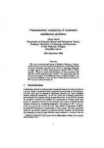
Representation Sets of Tuples DNF

CSP complexity O(m log(m)) O(m log(m))

Meta-problem complexity P coNP-complete

Figure 1: The complexity of the CSP for intersection-closed constraints and the complexity of the meta-problem, depending on the representation of the relations, where m denotes size of the input.

is called a-valid if a is an element of Γ and every relation in Γ contains a tuple of the form (a, . . . , a). Corollary 26. Unless P=NP, an equality constraint language with template Γ is tractable if and only if Γ is a-valid for some (equivalently, all) a ∈ Γ or if all relations can be defined by Horn =-formulas. Proof. By Lemma 8, the statement directly follows from Theorem 1. The presented algorithm for intersection-closed equality constraint languages does not only apply to finite constraint languages, but also to constraint languages where the constraints in the input are represented by sets of tuples or by DNF formulas. In the special case that the input contains intersection-closed constraints that are represented by Horn clauses, a resolution-based algorithm by Nebel and B¨ urkert can be applied as well; however, our algorithm has a significantly better running time. Our algorithm also outperforms algorithms that are based on establishing relational consistency. Finally, we also showed that the complexity of the problem to decide whether a given constraint language is tractable or not (assuming P 6= NP) depends on the way the constraint language is represented, and is either tractable for representations by sets of tuples, or coNP-complete for representations by DNF formulas. It is not hard to see that the P-complete problem of Horn-Sat (a boolean constraint satisfaction problem; see e.g. [10]) can be reduced to intersectionclosed equality constraints. Hence, the constraint satisfaction problem for the set of all intersection closed equality constraint is among the hardest problems of the complexity class P. An interesting question for future research is a more detailed study of the complexity of the equality constraint languages whose CSP is in P. For boolean constraint satisfaction problems, an analogous project was recently completed in [1]; it turned out that all boolean CSPs in P are P-complete, NL-complete, parity-L-complete, or in L. We would like to conclude with a remark on the relationship of the presented results with questions from universal algebra. The lattice of clones that contain all the permutations is a recent research focus in universal algebra [14, 19–21], and a full classification seems to be out of reach. However, the lattice of locally closed clones that contain the set of all permutations Sω is considerably simpler. The lattice has a smallest element, the clone that is locally generated by Sω . Above this clone the lattice has exactly two minimal clones that correspond to

22

the maximally tractable equality constraint languages. Is it possible to give a full description of the locally closed clones that contain all the permutations? Acknowledgements. We thank the anonymous referees of the conference and the journal version of the paper, and Nadia Creignou for helpful comments on the meta problem for boolean CSPs.

References [1] E. Allender, M. Bauland, N. Immerman, H. Schnoor, and H. Vollmer. The complexity of satisfiability problems: Refining Schaefer’s theorem. Electronical Colloquium on Computational Complexity, 2004. [2] M. Bodirsky. Constraint satisfaction with infinite domains. PhD thesis, Humboldt-Universitat zu Berlin, 2004. [3] M. Bodirsky and V. Dalmau. Datalog and constraint satisfaction with infinite templates. In Proceedings of the 23rd International Symposium on Theoretical Aspects of Computer Science (STACS’06), LNCS 3884, pages 646–659. A journal version is available from the webpage of the first author, 2006. [4] M. Bodirsky and J. K´ ara. The complexity of equality constraint languages. In Proceedings of the International Computer Science Symposium in Russia (CSR’06), LNCS 3967, pages 114–126, 2006. [5] M. Bodirsky and J. Neˇsetˇril. Constraint satisfaction with countable homogeneous templates. Journal of Logic and Computation, 16(3):359–373, 2006. [6] V. G. Bodnarˇcuk, L. A. Kaluˇznin, V. N. Kotov, and B. A. Romov. Galois theory for post algebras, part I and II. Cybernetics, 5:243–539, 1969. [7] A. Bulatov, A. Krokhin, and P. G. Jeavons. Classifying the complexity of constraints using finite algebras. SIAM Journal on Computing, 34:720–742, 2005. [8] P. J. Cameron. Oligomorphic Permutation Groups. Cambridge University Press, 1990. [9] D. Cohen, P. Jeavons, P. Jonsson, and M. Koubarakis. Building tractable disjunctive constraints. J. ACM, 47(5):826–853, 2000. [10] N. Creignou, S. Khanna, and M. Sudan. Complexity Classifications of Boolean Constraint Satisfaction Problems. SIAM Monographs on Discrete Mathematics and Applications 7, 2001. [11] R. Dechter and P. van Beek. Local and global relational consistency. TCS, 173(1):283–308, 1997. 23

[12] Garey and Johnson. A Guide to NP-completeness. CSLI Press, Stanford, 1978. [13] D. Geiger. Closed systems of functions and predicates. Pacific Journal of Mathematics, 27:95–100, 1968. [14] L. Heindorf. The maximal clones on countable sets that include all permutations. Algebra Universalis, 48:209–222, 2002. [15] W. Hodges. A shorter model theory. Cambridge University Press, 1997. [16] M. Krasner. G´en´eralisation et analogues de la th´eorie de Galois. Congr´es de la Victoire de l’Ass. France avancement des sciences, pages 54–58, 1945. [17] B. Nebel and H.-J. B¨ urckert. Reasoning about temporal relations: A maximal tractable subclass of Allen’s interval algebra. Journal of the ACM, 42(1):43–66, 1995. [18] T. Ottmann and P. Widmayer. Algorithmen und Datenstrukturen. Spektrum Akademischer Verlag, 2002. [19] M. Pinsker. Maximal clones on uncountable sets that include all permutations. Algebra Universalis, 54(2):129–148, 2005. [20] M. Pinsker. The number of unary clones containing the permutations on an infinite set. Acta Sci. Math. (Szeged), 71:461–467, 2005. [21] M. Pinsker. Maximal clones on uncountable sets that include all permutations. Semigroup Forum, 2007. Accepted for publication. [22] R. P¨ oschel and L. A. Kaluˇznin. Funktionen- und Relationenalgebren. Deutscher Verlag der Wissenschaften, 1979. [23] A. Szendrei. Clones in universal Algebra. Seminaire de mathematiques superieures. Les Presses de L’Universite de Montreal, 1986. [24] L. Valiant and V. Vazirani. Np is as easy as detecting unique solutions. In Proc. ACM Symp. on Theory of Computing, 1985.

24