The Complexity of Live Sequence Charts - Semantic Scholar

The Complexity of Live Sequence Charts Yves Bontemps? and Pierre-Yves Schobbens Institut d’Informatique, University of Namur rue Grandgagnage, 21 B5000 - Namur (Belgium) {ybo,pys}@info.fundp.ac.be

Abstract. We are interested in implementing a fully automated software development process starting from sequence charts, which have proven their naturalness and usefulness in industry. We show in this paper that even for the simplest variants of sequence charts, there are strong impediments to the implementability of this dream. In the case of a manual development, we have to check the final implementation (the model). We show that centralized model-checking is co-NP-complete. Unfortunately, this problem is of little interest to industry. The real problem is distributed model-checking, that we show PSPACE complete, as well as several simple but interesting verification problems. The dream itself relies on program synthesis, formally called realizability. We show that the industrially relevant problem, distributed realizability, is undecidable. The less interesting problems of centralized and constrained realizability are exponential and doubly-exponential complete, respectively.

1

Introduction

Scenario-based approaches and their supporting languages, by which we mean languages such as Message Sequence Charts (MSC) [1], UML Interaction Diagrams [2] or Live Sequence Charts (LSC) [3], have shown a clear advantage on other languages, in practice [4, 5]. They are simple, with a concrete semantics, and have some graphical appeal, which gives them a steep learning curve even for non-expert users. They are specially useful for distributed reactive systems, our focus here. Their apparent simplicity made most practitioners and theoreticians believe that all problems associated to these languages would be easy. A first blow to this commonly held belief was given by Muscholl et al. [6] who showed that several simple problems on HMSC are undecidable. Here, we show that many simple problems on (non-hierarchical) LSC have a surprisingly high complexity, and especially that the main tenet of the dream, the automated synthesis of a distributed algorithm, is undecidable. This may seem to render our dream unachievable, but actually it is hardly surprising that distributed software development, that requires the brains of millions of programmers worldwide and in which still today unexpected bugs are found, is undecidable. This means that more knowledge has to be put in the synthesis ?

FNRS Research Fellow

algorithms, e.g. as heuristics [7]. Thus although the dream will never be fully achieved, we can try to come close enough to it to alleviate the work of programmers of distributed systems. Thus, one can hope that synthesis will be hard in theory but usable in practice, as verification [8]. The paper is structured as follows. We present, in Sec. 2.1, the syntax and semantics of Live Sequence Charts (LSC), which is used to specify the future system behaviour. Design models of the system are given using an agent-oriented state-based formalism, here input/output automata, encoding strategies, as presented in Section 2.2. This section concludes by defining when a design model is a correct implementation of a scenario-based specification. In Sec. 3, verification problems are considered. First, checking whether a design model is a correct implementation (Sec. 3.1) and then, whether a specification refines another specification (Sec. 3.2). The question of whether a specification is implementable is investigated in Sec. 4. Sec. 5 presents various constructs that can be added to our version of LSCs, making the language more expressive, but preserving all the results of this paper. Finally, in Sec. 6, we summarize the results and put them in perspective.

2

Models

We assume that we are given a finite set of agents or processes Ag and of message names M. An event is a triple from Ag × M × Ag. The set of events is Σ. We will denote events sent (resp. received) by some agent a with Σas (resp. Σar ) and let Σa = Σas ∪ Σar . An event of the form (a1 , m, a2 ) represents the fact that a1 sends message m to a2 . We assume here, for simplicity, that communication is instantaneous. (In contrast, some undecidability proofs of [6] require the more complex FIFO communication). From agents behaviour emerge observable sequences of events. We identify behaviour and sequences of events. Σ ∗ represents the set of all finite sequences of events, while Σ ω are all infinite sequences. 2.1

Live Sequence Charts

Live Sequence Charts (LSC) [3] is based on Message Sequence Charts (MSC) [1]. LSCs present agents interactions. Every agent owns a “life-line”, labeled by its name, e.g. “ui”, “cm”, “client1” in Fig. 1. Interactions take place through events, that are shown as arrows. An occurrence of (a1 , e, a2 ) is displayed as an arrow labeled by m, from a1 ’s life-line to a2 ’s life-line. MSCs are unclear with respect to the “status” of a scenario, i.e. whether a scenario represents all possible behaviours or just some of them. They are also silent about the role of messages that do not appear in a scenario, viz. whether they are forbidden by their mere absence or whether they can appear at will. We call this feature message abstraction. Furthermore, engineers informally assign different statuses to messages: some of them trigger the described scenario, whereas other are expected answers.

LSC clarifies this [3]. Syntactic constructs are added to MSCs to state explicitly whether the diagram is a mere example (existential scenarios) or constrains all behaviours of the future system (universal scenarios). The former are simply MSCs, surrounded by a dashed-line box. The latter are MSCs, divided in two parts: an upper part, named prechart, that is graphically surrounded by an hexagonal dashed-line box, and a lower-part, called main chart, surrounded by a solid-line rectangle. The intuitive semantics is “whenever the agents behave as in the prechart, they shall behave according to the main chart afterwards”. LSC adds “message abstraction” by explicitly stating which events are restricted. All events appearing in the LSC are automatically restricted. Additional events can be restricted thanks to a “restricts” clause. This provides the scenario with a scope (alphabet). Like MSCs, their semantics is based on a partial order. To be fully rigorous, the partial order is the equivalence class quotient of the preorder defined by rules (1-3) below. The temporal ordering of events is deduced from three constraints and their transitive closure: (1) life-lines induce a total ordering on their events, from top to bottom, (2) agents synchronize on shared events, i.e. two locations linked by an arrow are order-equivalent and (3) all locations in the prechart appear before main chart locations. In MSC parlance, the prechart and main chart are strongly sequenced. For example, combining the clauses, in Fig. 1, events “getdata” and “updating” are unordered. Clause (1) can be relaxed thanks to co-regions. A co-region is a sequence of locations, belonging to the same life-line, along which a dashed line is drawn, see the two “getnew” events in Fig. 1.

ui

cm

client1

client2

db

update

getnew getdata getnew updating

getdata

Fig. 1. Update Scenario

Live Sequence Charts have been used to model various real-life systems such as the weather synchronization logic of NASA’s Center TRACON Automation System (CTAS) [9], a radio-based train system [10], virtual wrappers for PCI bus [11] and some part of the C elegans worm [12]. Examples displayed in Fig. 1 and 2(a) and (b) are based on the CTAS system. This system aims at synchronizing various clients that make use of weather reports. When new forecasts are available, a protocol is followed to update clients data. If some client fails to update, they try to roll back to the previous consistent state. The rationale is that all clients should always be using the same data. The following requirements are described by LSCs.

1. When the user asks for an update, all clients are asked to fetch the new weather reports. The user is notified of the updating process. See Fig. 1. 2. If some client fails to update its state, all clients are required to roll back to the previous state, after the user has been notified that the updating process is taking place. See Fig. 2(a). 3. Whenever the database refuses a download, the cm (communication manager) is notified. See Fig. 2(b).

ui

cm

client1

client2

cm

client1

db

update

getdata getnew failure

nack

updating

useold

failure useold

failed

(a)

(b) Fig. 2. Failure scenarios

We now define formally the abstract syntax and the semantics of universal LSCs. It is based on labeled partial orders. Definition 1 (Labeled partial order (LPO)). Let V be a set of events. A V -labeled partial order (V -LPO) is a tuple hL, ≤, λ, Σ 0 i, where L is a set of locations. If L is finite, the LPO is called finite. ≤⊆ L × L is a partial order on L (a transitive, anti-symmetric and reflexive relation). λ : L → V is a labeling function. A linearization of a finite LPO is a word of w1 . . . wn ∈ Σ ∗ such that the LPO h[n], ≤, {(i, wi )|i ∈ [n]}i, where [n] is a shortcut for the set {1, . . . , n}, is isomorphic to some linear (total) order hL, ≤0 , λi with ≤⊆≤0 . A labeled partial order represents an MSC. As already stated above, LSC distinguishes between examples (existential LSC) and request-reply rules (universal LSC), in which the activation part is singled out. Definition 2 (LSC). Universal LSC. A universal LSC is a tuple hL, ≤, λ, ΣR , P i such that 1. hL, ≤, λi is a finite ΣR -LPO. ΣR are called the restricted events of the LSC; 2. P ⊆ L is called a prechart. Main chart locations are all larger than prechart locations: P × (L \ P ) ⊆≤. Existential LSC. An existential LSC is a tuple hL, ≤, λ, ΣR i such that hL, ≤, λi is a finite ΣR -LPO.

We will be considering infinite words γ ∈ Σ ω . A word γ is a model of an LSC if, at any point in γ, if the prechart is linearized, then the main chart is also linearized afterwards. Definition 3 (γ |= S). For every γ = e0 e1 . . . ∈ Σ ω , γ |= S iff S is a Universal LSC and ∀i ≥ 0 : (∃j ≥ i : ei . . . ej |ΣR linearizes P ) ⇒ (∃k ≥ i : ei . . . ek |ΣR linearizes L) S is an Existential LSC and ∃i ≥ 0 : ∃j ≥ i : (ei . . . ej )|ΣR linearizes L The size of an LSC is its number of locations. An LSC specification is a set of universal LSCs, the semantics of which is defined by conjunction; a run is a model of an LSC specification iff it is a model of all its constituent scenarios. The size of a specification is the sum of the size of the conjuncted LSCs. The language defined by an LSC is its set of models: L(L) = {γ ∈ Σ ω |γ |= L}. Every LSC specification is equivalent to the conjunction of liveness and safety properties, one for every event in Σ [13]. A scenario S, with restricted events ΣR , forbids e ∈ Σ after a finite run w ∈ Σ ∗ iff some suffix of w|ΣR , say w0 , linearizes an ideal I of the LSC, which includes P , but w 0 · e does not linearize any ideal in S. S requires e ∈ Σ iff some suffix w 0 of w|ΣR linearizes an ideal I ⊇ P of S and w0 · e is a linearization of some ideal in S. An infinite run γ ∈ Σ ω is e-safe iff for every prefix w of this run, if e is forbidden by some scenario after w, w · e is not a prefix of γ. It is e-live iff for every prefix w of γ, if some scenario requires e after w, then e eventually occurs after w. Theorem 1 (LSC = Live + Safe). An infinite run γ ∈ Σ ω satisfies an LSC specification iff, for every e ∈ Σ, γ is both e-safe and e-live [13]. 2.2

Strategies

Agents are partitioned into two teams: the environment and the system. Formally, Ag = Sys ∪˙ Env. System-controlled events are ΣSys = Sys × M × Ag. Engineers are not asked to construct programs for agents in Env, only agents from Sys have to be implemented. Sys implementation will be deployed among Env agents that provides thus the model-time context of the specification. We will use Input/Output automata to describe the design-time model of agents [14]. An input-output automaton for agent a ∈ Ag is a finite automaton the alphabet of which is Σa . A distinction is made between input events (Σar ) and output events (Σas ) Syntactically, an I/O automaton for agent a must be input-enabled: for every input event e ∈ Σar , in every state q, there is an outgoing transition labeled by e. In other words, a may never block incoming messages. A run of an I/O automaton is an infinite path in the automaton, following the transition relation and starting from the designated initial state. A fair run is a run in which infinitely many transitions labeled by Σas events are taken. The

word generated by a run is the infinite sequence of events encountered along the transitions of the run. The language of an I/O automaton A, denoted L(A), is the set of words generated by A’s fair runs. The composition of two I/O automata (A1 × A2 ) is defined as the synchronous product of A1 and A2 , see [14] for details. A finite state I/O automaton represents a finite-memory strategy for agent a. s Formally, a (non-deterministic) strategy for agent a is a function f : Σ ∗ → 2(Σa ) . It is of finite memory if there is an equivalence relation ' on Σ ∗ such that (1) ' is of finite index and (2) ∀w ' w 0 : f (w) = f (w0 ). The size of the memory is the index of the smallest such equivalence relation. Clearly, every finite memory strategy can be translated to an I/O automaton. Conversely, every I/O automaton can be turned into a strategy. The outcome of a strategy f is the set of all runs in which Σas events appear only according to the strategy. Out(f ) = {u0 e0 u1 e1 . . . |∀i ≥ 0 : ui ∈ (Σ \({a}×M×Ag))∗ ∧ei ∈ f (u0 e0 . . . ui )}. Definition 4 (Correct Implementation). A design model M , presented as a list of strategies (fa )a∈Sys , T is a correct implementation of an LSC specification iff, for every outcome w ∈ a∈Sys Out(fa ), – if w is ΣEnv -live, then w is ΣSys -live; – and if w is ΣEnv -safe, then w is ΣSys -safe.

3 3.1

Verification Model Checking

The first problem we consider is the verification that a closed and centralized implementation is correct. This problem makes two assumptions: there are no environment agents, thus all agents described in the LSC are system agents and their behaviour is specified thanks to a single automaton. Definition 5 (CCMC). Closed Centralized Model Checking (CCMC) is, given an automaton A and an LSC specification {L1 , . . . , Ln }, to decide whether T L(A) ⊆ ni=1 L(Li ). This problem is co-NP complete. A first extension is to consider that some agents belong to the environment, while others are system agents. Then, we are presented with an implementation of system agents only and the question becomes: “whenever environment agents do behave correctly, does this implementation behave appropriately?”. The problem becomes PSPACE-complete. Definition 6 (OCMC). Open Centralized Model Checking(OCMC) is, given an automaton A, a partition of Ag into Sys and Env and an LSC specification S, to decide whether A is a correct implementation of Sys with respect to S (see def. 4).

The second restriction imposes that we consider monolithic systems only, made of a single component. As it was clear from the introduction, we are mostly interested in distributed systems. The design-time specification of such systems will typically be presented as a “network” of automata, one for each agent. Every automaton prescribes how its owner shall behave, see Sec. 2.2. Definition 7 (Closed Distributed Model Checking). Given an LSC L Qk and a list of automata (Ai )i=1,...,k , decide whether L( i=1 Ai ) ⊆ L(L). Unfortunately, as usual in verification [15], this makes model checking more complex. The problem becomes PSPACE-complete instead of coNP-complete. Combining distribution and openness does not increase the problem complexity; it is still PSPACE-complete. Theorem 2. CCMC is complete for coNP. CDMC, OCMC and ODMC are PSPACE-complete. Proof. CCMC coNP-hardness is shown by reducing the complement of the Traveling Salesman Problem (coTSP) to CCMC. coTSP is to decide whether in a given weighted directed graph, all circuits have a total weight of larger than a given bound k. One can restrict to edge weights ≤ 2 [16]. The graph and the cost are encoded in the automaton with a counter: (1) when an edge of weight j is followed to a vertex v, the counter is incremented by j and an event v is emitted. At any point, the counter can be down-counted: if the counter is at n, n “billing” events are omitted and a final “zero” event follows. An LSC is added, the prechart of which states that all vertices should be visited once, in any order, and the main chart imposes that k “billing” events without any “stop”. PSPACE-proofs of open systems use the same technique as LSC-Reach (see below). PSPACE-proof of distributed variants rely on the fact that deadlock detection in a network of processes is PSPACE-complete [16]. All membership proofs are standard: a violating simple path is guessed in the automaton and it is checked that it actually violates the LSC. The complexity of this procedure follows from an argument on the length of simple paths in LSC tableau automata. One can believe that this high complexity is due to the presence of automata in the problems, as sketched by the proof of Th. 2. The next section presents simple analysis problems, on LSCs only, that are also difficult. This is astonishing, as one might think that these problems can be solved by easy computations on the diagrammatic form of LSCs. 3.2

Reachability and Refinement Checking

The first problem we consider is whether an LSC specification allows some use case. Definition 8 (LSC-Reach). LSC Reachability (LSC-Reach) is, given an exU istential LE and an LSC specification {LU 1 , . . . , Ln }, to decide whether Tn LSC u E ∃γ ∈ i=1 Li : γ |= L .

LSC-Reach checks that a certain specification, together with assumptions over the domain still makes it possible to achieve a certain behaviour. This problem is PSPACE-complete. Another natural problem on LSC only is verifying specification refinement is al. Given a certain abstract specification S, a more precise specification S 0 is designed and we want to verify that every behaviour induced by S 0 is a legal behavior of S. Logically, this boils down to verifying the validity of S 0 → S. This problem is also PSPACE-complete. Definition 9 (LSC-Impl). LSC Implication (LSC-Impl) is, given two LSC specifications S and S 0 , to decide whether L(S 0 ) ⊆ L(S). Theorem 3. LSC-Reach and LSC-Impl are complete for PSPACE. Proof. PSPACE-hardness is obtained from reducing the halting problem of a PSPACE TM on the blank input to LSC-Reach. We sketch our encoding of a DPSPACE TM configuration, with the additional assumptions that (1) the halting configuration is never left and (2) when the halting configuration is reached, the tape head is moved to the leftmost tape cell. A TM configuration is of the form (γ, i, T ) where γ ∈ Γ is a control state, 0 ≤ i ≤ n is the tape head position (remark that at most n cells are used, this is known a priori) and T [j] ∈ {0, 1} (0 ≤ j ≤ n) is the tape content. The vocabulary of our LSC specification is (Γ ∪ {in, $} ∪ {0, 1}) × {0, . . . , n}. The symbol in is used to initialize the TM simulation: when it occurs, an initial configuration is output and $ is a technical marker, we skip its description here. A TM configuration is encoded by a word w if 1. ∃v : w = v(γ, i) 2. ∀j : 1 ≤ j ≤ n : T [j] = a ⇒ ∃u, v : w = u(a, j)v and neither (0, j) nor (1, j) appears in v. We have to describe the encoding of the TM transition relation. Suppose, wlog, that C = (T, γ, i), T [i] = 0 and C 0 = (T 0 , γ 0 , i + 1), where T 0 is like T , except that 1 has been written at the i-th position. Assume that C is encoded by some word w. By definition of configuration encoding, w = v · (γ, i), and the last occurrence of either {(0, i), (1, i)} is (0, i) in w. The transition will be encoded as the following continuation: w0 = v (γ, i)(0, i)($, i)(1, i)(γ 0, i + 1) . {z } | u

One can check that w 0 is indeed an encoding of C 0 , by noting that 1. it ends with (γ, i + 1); 2. in u, no event of the form (0, j) or (1, j) (j 6= i) has been added. Hence, the tape content of the configuration encoded by w does not differ from that of C on these cells.

These rules can be described by universal LSCs and the existential LSC is simply there to ensure that, in at least one run, in occurs and later on in the same run, the halting location appears, too. Harel and Marelly introduced an algorithm and an approach to the validation of LSC-based specifications, called play-out [17]. The specification is immediately executed, without generating any code from it, but using an animation engine instead. This animation engine uses a superstep approach: when the environment inputs some new event, by performing some action on the graphical user interface, the engine performs all system-controlled events that become required, until it reaches some stable status, in which no event is required anymore. The theorems provided in this section can be adapted to show that computing whether a finite super-step exists is PSPACE-complete. Smart play-out is a practically efficient technique that uses symbolic model checking of LTL formulae to discover such a superstep [18].

4

Realizability

In this section, we turn to the most complex class of problems considered in this paper. We want to determine automatically whether a specification is implementable. Ideally, the proof of implementability should be constructive: some state-based implementation of the specification must be built. Would this implementation be compact and readable, the burden of designing the system would be taken away from engineers. We are interested in implementing open reactive systems. As noted by [19] and [20], realizability is not equivalent to satisfiability. Actually, the question is more accurately posed as “is there an implementation of system agents such that, no matter how environment agents behave, the specification will be respected?”. We will first assume that system agents are built under the “perfect information” hypothesis. This artificial hypothesis implies that system agents may observe every event and that every system agent knows instantaneously in what state other agents are. Then, we will see that dropping this hypothesis implies undecidability of realizability. Definition 10 (CR). Centralized Realizability (CR) is, given an LSC specification {L1 , . . . , Lm } and a set of system agents Sys ⊆ Ag, to decide whether s , such that f is a correct implementation of there is a strategy f : Σ ∗ → ΣSys {L1 , . . . , Lm }. In [13], we have presented an exponential time algorithm solving this problem. It constructs a two-player parity game graph, with three colors, in which player 0 has a winning strategy iff the specification is realizable. The game graph is exponentially larger than the LSC specification. This problem is EXPTIME-complete. This proves our claim that, because LSCs are less expressive than LTL, some problems are easier on LSCs than on LTL. Actually, centralized realizability is 2EXPTIME-complete for LTL [20].

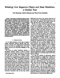
The algorithm presented in [13] is computationally expensive, yet optimal. However, it suffers from another problem: it yields design models, as automata, that are exponentially larger than the specification. This is a hindrance for readability. Nevertheless, we show below that strategies realizing LSC specifications need memories that large. Therefore, our algorithm is optimal, in the sense that every algorithm solving this problem will necessarily build exponentially large implementations. We exhibit in Fig. 3 a family of LSC specifications (φn )n>0 the size of which grows quadratically in n but any strategy for Sys realizing φn needs at least 2n log n memory states.

Env

Sys

a1

. . .

Env

Sys

ai

an ak

$ $

b1

. . .

bi

bn

bk

i 6= k and i, k ∈ {1, . . . , n}. Fig. 3. LSC specification φn

s r In this game, Env controls {a1 , . . . , an } = ΣEnv = ΣSys and Sys controls s r {$, b1 , . . . , bn } = ΣSys = ΣEnv . Env first presents Sys with a sequence of n symbols. Remark that Env chooses the order in which those events occur. When the whole sequence has been presented, Sys must reply with the same sequence. Hence, Sys’s strategy must have at least enough memory to remember the order in which the n events have been presented, viz. nn states. The LSC specification encoding this game is presented in Fig. 3. Along “Sys” and “Env” on the lefthand side scenario, we drew two dashed lines. This defines a co-region, which relaxes the ordering on the enclosed events. Therefore, a1 . . . an can occur in any order, see Section 2.1. In comparison, on the right-hand side, ai and ak are ordered. The right-hand side scenario obliges bi to follow bk if ak occurred after ai .

Theorem 4 (Memory Lower-Bound). There is a family of LSCs specification, namely (φn )n>0 such that any strategy realizing φn has a memory of size 2Ω(n log n) . Proof. First of all, for every n |φn | = 5n2 + 3n + 1. Hence, the size of φn grows only quadratically in n.

s Now, consider some strategy f : Σ ∗ → ΣSys winning in this game. If f is a correct implementation, it must have enough memory to remember the order in which a1 . . . an occurred. Otherwise, there would exist two words w and w 0 s s of (ΣEnv )∗ such that every symbol of ΣEnv occurs exactly once in both w and w0 , w 6= w0 , and f has not enough memory to distinguish w and w 0 , i.e. w ' w0 , and thus f (w) = f (w 0 ) (see Sec. 2.2). Therefore, w · f (w) = w · f (w 0 ) and consequently, f would not be winning, since the order of replies (b’s) does not match the order of queries (a’s). Contradiction. All permutations of a1 . . . an are possible, therefore there must be as many memory states in f as there are permutations of n elements, i.e. 2Ω(n log n) .

Remark 1 (Succinctness). Using the same family of LSC specifications and the same proof, one can show that translating LSCs to some DBA involves an exponential blow-up. Actually, it is not even possible to translate LSCs to NBA recognizing either the language of the specification or its complement without this blow-up. It follows from this fact and from the theorems in [21] that turning LSCs to equivalent ACTLdet formulae also involves an exponential blow-up. Indeed, for every ACTLdet formula, there is a nondeterministic B¨ uchi automaton recognizing their complement, which is linear in their size. The problem of centralized realizability is lacking some features, which lessens its applicability 1. It would be interesting to come up with an implementation that satisfies the specification and guarantees that additional requirements will be met as well. This is especially interesting if the specification is too abstract or too loosely defined to ensure the requirements, but the analyst thinks that it is possible to refine it in a way that would fulfill the requirements. The problem of deciding whether there is such a particular implementation, which we call Constrained Realizability is 2EXPTIME-complete, when we consider LTL as a language for expressing requirements. 2. It does not take the structural model into account, because it assumes that the “perfect information” hypothesis holds. Hence, agents are not obliged to consider only events occurring at their interfaces. It seems necessary to extend the centralized version of the problem to take this into account. This variant is called Distributed Realizability (DR). As for LTL, this problem is undecidable [22]. The proof of this theorem, given in appendix, is similar to the proof presented in [23], to show that the problem of decentralized observation is undecidable. The problem of distributed realizability is, intuitively, to determine whether there is a network of implementations, in which every agent only senses events at its interface but the composition of which implements the specification. Distributed realizability becomes undecidable, Definition 11 (DR). Distributed Realizability (DR) is, given an LSC specification {L1 , . . . , Lm }, to decide whether there is a list of strategies (fa )a∈Sys one for every system agent, such that

1. fa : Σ ∗ → (Σas ); 2. ∀w, w0 ∈ Σ ∗ : w|Σa = w0 |Σa ⇒ f (w) = f (w 0 ), i.e. if w and w0 are the same, from a’s point of view, then a shall behave the same way after w or w 0 ; T 3. a∈Sys Out(fa ) is a correct implementation of {L1 , . . . , Lm }. Theorem 5. CR is EXPTIME-complete and DR is undecidable. Proof. EXPTIME-hardness of CR is obtained from the reduction of the halting problem of an alternating PSPACE TM to CR. The reduction is similar to the one provided in the proof of Th. 3. TM alternation is mapped on the statuses (antagonist vs protagonist) of the environment and the system. Post’s Correspondence Problem (PCP) can be reduced to DR, hence showing that DR is undecidable. The proof is essentially the one proposed by Tripakis [23]. Let us fix an arbitrary PCP instance (w1 , u1 ) . . . (wn , un ) over some alphabet Θ. The alphabet of our LSC specification is Θ ∪ {k1 , . . . , kn } ∪ {$} ∪ {0, 1} ∪ {A0 , A1 }, plus an arbitrary finite number of events which can be exchanged between system agents, say {s0 , . . . , sq }. The system is made of two agents: a1 and a2 . The first agent may observe Θ ∪ {$}, whereas the second can observe {k1 , . . . , km , $}. All these events, but {A0 , A1 } and the additional system events {s0 , . . . sk } are controlled by the environment. A play proceeds as follows. First, the environment picks either 0 or 1. The former means that the environment chooses to read words in the first component of the pairs of words (viz. the wi ’s), the latter means that it will read ui ’s. Then, the environment must stick to that choice until the end of the play. Namely, the environment chooses a particular word in the list (say, wi or ui , depending on the “column” chosen) and indicates the index of this word to the system, by performing ki . The environment must enumerate the letters in wi , which are published to agent a1 . The game goes on until the environment performs $. At this point, the system is required to output A0 or A1 , depending on what index (0 or 1) the environment had chosen in the first place. We claim that the PCP instance has a solution iff this specification is not implementable. Assume that PCP has a solution i1 . . . im but there is a winning strategy for the system. Then, upon 0i1 w1 . . . im wm $, the system answers with A0 . The strategy of the system shall also answer A0 to A1 i1 ui1 . . . im um $, because the projections of the two words on agent’s alphabets are the same. Therefore, there is no winning strategy. If the PCP instance has no solution, then, the two system agents can get together and compare the submitted run. Agent a2 sends the sequence of indices that it has been presented with to a1 (using some protocol on which they agreed, based on {s0 , . . . , sp }). This agent can then build wi1 . . . wim and compare it with the word that he has received from the environment. Since the PCP instance has no solution, either they are the same and a1 shall answer A0 or the two words differ and a1 replies with A1 .

5

Extensions

The language of LSC that we have used so far was pretty simple. In this section, we present some possible extensions, that make it more expressive but does not cause any changes in the complexity of the problems investigated in this paper. Actually, all membership proofs can be simply adapted to deal with these extensions. Hardness proofs are of course not affected by adding new constructs to the language. Alternatives: within a single LSC, one can describe several alternatives, as is done with inline constructs of MSCs or Sequence Diagrams. We need to introduce the concept of LPOs with choice, which is much heavier to manipulate. This extension does not cause any other problem, as the tableau automaton of the LSC remains simply exponential. Conditions: it is possible to add conditions (i.e. boolean logic over some predefined set of propositions), to the language. Together with alternatives, we can embed if-then-else tests in the language. Using the concept of cold/hot conditions, one can also describe some “preconditions” and assertions: a hot condition describes a condition that must be true when it is evaluated, whereas a cold condition represents a condition that, if evaluated to false, finishes prematurely and successfully the scenario. Again, all the results of this paper remain true if we consider this extension. Hot/Cold Locations: a cold location is a location on which the execution of the chart may stop. This provides us with a way to specify that some linearizations of the LPO may stop before reaching its end. Modes of communication: In our model, we assumed that communication was instantaneous. Nevertheless, we can represent other modes of communication, like asynchronous or synchronous communication in our model. Asynchronous communication means that the receiver shall not be ready for the sender to send its message. In the synchronous mode, there is a transmission delay, too, but the sender must wait for the receiver to get the message before proceeding. This represents procedure calls, in programming languages. Unbounded loop is the only extension for which we could not prove the robustness of our constructions. With the Kleene star and alternatives, we can encode every regular expression as a basic chart. We were not able to show that the double blow up involved in the tableau method could be avoided, and we leave that problem open. Remark that Kleene star makes the language incomparable to LTL.

6

Summary and Discussion

There are two axes along which complexity increases. The distributed version of the problems is always harder than the centralized one, as in [15], while synthesis

is also more complex than model checking, for it adds alternation to the problem [24]. The most interesting part is to investigate what causes such a high complexity. We identify two factors making LSCs complex. 1. LSC semantics relies on partial orders. We used this in the proof of coNP-completeness of CCMC (Th. 2) and the lower-bound on the size of synthesized state machines (Th.4). With a chart of size n, we can thus encode a set of runs of exponential size. 2. An LSC specification is unstructured. In the PSPACE-hardness proofs, we used LSCs of constant size only and, actually, very short ones, in which events were linearly ordered. The complexity of the specification comes from the fact that many LSCs are active at the same time, describing concurrent liveness properties. The former cause of complexity is often avoided in practice, because realworld specifications tend to consist of almost linearly ordered scenarios. The latter cause is more difficult to deal with. One shall find ways to describe the problem structure in these models and, more importantly, to rely on this additional information to get more efficient algorithms. This is all but an easy task, as it contradicts one of the basic principles of scenario-based software engineering: requirements are partial, redundant, complementary and range over several aspects of the system. Undecidability of distributed synthesis means that we need to find other ways to cope with that problem. In [7], we propose such an algorithm, which is sound but not complete. It applies a predefined “implementation scheme” and then checks whether the distributed implementation obtained is correct.

References 1. International Telecommunication Union (ITU) Geneva: MSC-2000: ITU-T Recommendation Z.120 : Message Sequence Chart (MSC). (2000) http://www.itu.int/. 2. Object Management Group (UML Revision Task Force): OMG UML Specification (2.0). (2003) http://www.omg.org/uml. 3. Damm, W., Harel, D.: LSCs: Breathing life into message sequence charts. Formal Methods in System Design 19 (2001) 45–80 4. Weidenhaupt, K., Pohl, K., Jarke, M., Haumer, P.: Scenario Usage in System Development: A Report on Current practice. IEEE Software 15 (1998) 34–45 5. Amyot, D., Eberlein, A.: An evaluation of scenarion notations for telecommunication systems development. Telecommunications Systems Journal 24 (2003) 61–94 6. Muscholl, A., Peled, D., Su, Z.: Deciding Properties of Message Sequence Charts. Foundations of Software Science and Computer Structures (1998) 7. Bontemps, Y., Heymans, P.: As fast as sound (lightweight formal scenario synthesis and verification). In Giese, H., Kr¨ uger, I., eds.: Proc. of the 3rd Int. Workshop on “Scenarios and State Machines: Models, Algorithms and Tools” (SCESM’04), Edinburgh, IEE (2004) 27–34

8. Harel, D.: From play-in scenarios to code : An achievable dream. IEEE Computer 34 (2001) 53–60 a previous version appeared in Proc. of FASE’00, LNCS(1783), Springer-Verlag. 9. Bontemps, Y., Heymans, P., Kugler, H.: Applying LSCs to the specification of an air traffic control system. In Uchitel, S., Bordeleau, F., eds.: Proc. of the 2nd Int. Workshop on “Scenarios and State Machines: Models, Algorithms and Tools” (SCESM’03), Portland, OR, USA, IEEE (2003) 10. Bohn, J., Damm, W., Klose, J., Moik, A., Wittke, H.: Modeling and validating train system applications using statemate and live sequence charts. In Ehrig, H., Kr¨ amer, B.J., Ertas, A., eds.: Proceedings of the Conference on Integrated Design and Process Technology (IDPT2002), Society for Design and Process Science (2002) 11. Bunker, A., Gopalakrishnan, G.: Verifying a VCI Bus Interface Model Using an LSC-based Specification. In Ehrig, H., Kr¨ amer, B.J., Ertas, A., eds.: Proceedings of the Sixth Biennial World Conference on Integrated Design and Process Technology, Society of Design and Process Science (2002) 48 12. Kam, N., Harel, D., Kugler, H., Marelly, R., Pnueli, A., Hubbard, J.A., Stern, M.J.: Formal modelling of c. elegans development; a scenario-based approach. In Ciobanu, G., Rozenberg, G., eds.: Modelling in Molecular Biology. Natural Computing Series. Springer (2004) 151–173 13. Bontemps, Y., Schobbens, P.Y., L¨ oding, C.: Synthesis of open reactive systems from scenario-based specifications. Fundamenta Informaticae 62 (2004) 139–169 14. Lynch, N.A., Tuttle, M.R.: An introduction to input/output automata. CWI Quarterly 2 (1989) 219–246 15. Harel, D., Vardi, M.Y., Kupferman, O.: On the complexity of verifying concurrent transition systems. Information and Computation 173 (2002) 16. Papadimitriou, C.H.: Computational Complexity. Addison-Wesley (1994) 17. Harel, D., Marelly, R.: Come, let’s play! Scenario-based programming using LSCs and the Play-engine. Springer (2003) ISBN 3-540-00787-3. 18. Harel, D., Kugler, H., Marelly, R., Pnueli, A.: Smart Play-Out of Behavioral Requirements. In: Proc. 4th Intl. Conference on Formal Methods in ComputerAided Design (FMCAD’02), Portland, Oregon. (2002) 19. Abadi, M., Lamport, L., Wolper, P.: Realizable and unrealizable specifications of reactive systems. In Ausiello, G., Dezani-Ciancaglini, M., Rocca, S.R.D., eds.: Automata, Languages and Programming, 16th International Colloquium, ICALP89, Stresa, Italy, July 11-15, 1989, Proceedings. Volume 372 of Lect. Notes in Comp. Sci., Springer (1989) 20. Pnueli, A., Rosner, R.: On the Synthesis of a Reactive Module. In: Proceedings of the sixteenth annual ACM symposium on Principles of programming languages. (1989) 179–190 21. Maidl, M.: The common fragment of CTL and LTL. In: Proc. 41st Annual Symposium on Foundations of Computer Science. (2000) 643–652 22. Pnueli, A., Rosner, R.: On the synthesis of an asynchronous reactive module. In Ausiello, G., Dezani-Ciancaglini, M., Rocca, S.R.D., eds.: Automata, Languages and Programming, 16th International Colloquium (ICALP). Volume 372 of Lect. Notes in Comp. Sci., Stresa, Italy, Springer-Verlag (1989) 652–671 23. Tripakis, J.: Undecidable problems of decentralized observation and control on regular languages. Information Processing Letters 90 (2004) 24. Chandra, A.K., Kozen, D.C., Stockmeyer, L.J.: Alternation. Journal of the ACM 28 (1981) 114–133