Mar 21, 2000 - However, usually these problems were defined using formulae or circuits with a com- plete base of boolean operations or gates, mostly with the ...
The Complexity of Problems Defined by Boolean Circuits - Preliminary Version -
Steffen Reith Klaus W. Wagner Lehrstuhl für Theoretische Informatik Universität Würzburg [streit,wagner]@informatik.uni-wuerzburg.de 21st March 2000
Keywords: Computational complexity, boolean circuits, circuit value problem, satisfiability, tautology, counting functions, threshold problem. Abstract We study the complexity of circuit-based combinatorial problems (e.g., the circuit value problem and the satisfiability problem) defined by boolean circuits with gates from an arbitrary finite base B of boolean functions. Special cases have been investigated in the literature. We give a complete characterization of their complexity depending on the base B . For example, for the satisfiability problem for boolean circuits with gates from B we present a complete collection of (decidable) criteria which tell us for which B this problem is in L, is complete for NL, is complete for �L, is complete for P, or is complete for NP. Our proofs make substantial use of the characterization of all closed classes of boolean functions given by E.L. P OST already in the twenties.
1
Introduction
The complexity of formula-based and circuit-based combinatorial problems was studied through the more than three decades of Complexity Theory. Already in 1971, S.A. C OOK [Coo71] proved that the satisfiability problem for boolean formulae is NP-complete: This was the first NP-complete problem ever discovered. R.E. L ADNER [Lad77] proved in 1977 that the circuit value problem is P-complete. In many cases when a new complexity class was introduced and investigated, a formula-based or circuit-based combinatorial problem was the first which was proved to be complete for this class (see [SM73, Gil77], for example). However, usually these problems were defined using formulae or circuits with a complete base of boolean operations or gates, mostly with the base f^; _; :g. But what about the complexity of such problems when a different base is used? There are several special results of this kind (e.g. [Sim75, Gol77, Lew78, GP86]). In particular, there are very detailed investigations for the special case of boolean formulae in conjunctive normal form in [Sch78, Cre95, CH96, CH97, KST97, KSW97, RV98]. But there are no results answering this question for unresricted circuits in full generality. In this paper we will give complete characterizations of the complexity of some combinatorial problems defined by circuits with boolean gates from an arbitrary finite base. The paper is organized as follows. In Section 2 we briefly introduce some notation and results needed from Complexity Theory. In Section 3 we define B -circuits as boolean circuits with gates from a finite set B of boolean functions, and we define BF[B ℄ as the class of boolean functions computed by B -circuits.
The complexity of a problem defined by B -circuits only depends on BF[B ℄. The classes of the form BF[B ℄ are exactly those classes of boolean functions which contain the identity function and which are closed under superposition (i.e., substitution, permutation of variables, identification of variables, and introduction of fictive variables). Already in the twenties, E.L. P OST [Pos41] gave a complete characterization of these classes. We make substantial use of his results which we present in Section 4. In Sections 5-9 we study the complexity of the circuit value problem, the satisfiability problem and the tautology problem, some quantified circuit problems, the counting function, and the threshold problem, resp., when defined by circuits with boolean gates from an arbitrary finite base B . We give complete characteriza(B ) be the set tions of their complexity as in the following example. Let the satisfiability problem of all B -circuits which evaluate to 1 for at least one input tuple. If B consists only of 1-reproducing (B ) is in functions, of self-dual functions, or of non-functions (for definitions see Section 4), then log L. Otherwise, if B consists only of and-functions or of or-functions then (B ) is �m -complete for NL. Otherwise, if B consists only of linear functions then (B ) is �log -complete for �L. Otherm log (B ) consists only of monotone functions then (B ) is �m -complete for P. Otherwise wise, if log (B ) is �m -complete for NP.
SAT
2
SAT SAT
SAT
SAT
SAT SAT
Complexity Theoretic Preliminaries
In this section we will informally introduce some standard notation and results from complexity theory. For more details see [BDG90a, BDG90b, Pap94]. The complexity classes P, NP, L, NL, and PSPACE are defined as the classes of languages (problems) which can be accepted by deterministic polynomially time bounded Turing machines, nondeterministic polynomially time bounded Turing machines, deterministic logarithmically space bounded Turing machines, nondeterministic logarithmically space bounded Turing machines, and deterministic polynomially space bounded Turing machines, resp. Let PP be the class of languages which are accepted by a nondeterministic polynomially time bounded Turing machine M in the following manner: An input x is accepted by M iff more than half of M ’s computation paths on input x are accepting paths. Let �L be the class of languages which are accepted by a nondeterministic logarithmically space bounded Turing machine M in the following manner: An input x is accepted by M iff the number of M ’s accepting paths on input x is odd. For a class K of languages let o-K =df fA j A 2 Kg. Furthermore let PK , NPK , LK , and NLK be the classes of languages accepted by the type of machines used for the classes P, NP, L, and NL, resp., but which have the additional ability to ask free-of-cost queries to languages from K (such machines are called p oracle machines). Define the classes of the polynomial time hierarchy by �p1 =df NP, �pk+1 =df NP�k , and �pk =df o-�pk for k � 1. Let FP be the class of functions which can be computed by a deterministic polynomially time bounded Turing machine. For a nondeterministic polynomially time bounded machine M let #M (x) be the number of accepting paths of M on input x. Let #P be the class of all such functions #M . For a class K of sets and a function s : N ! N , let FLK jj [s℄ be the class of all functions which are computable by a logspace bounded Turing machine which, for inputs of length n, can make at most s(n) parallel queries (i.e., the list of all queries is formed before any of them is asked) to a language from K. Here are some basic facts on the complexity classes defined above.
L � NL \ �L and NL [ �L � P � NP � PSPACE. All languages in NL [�L can be accepted by deterministic log2 n space bounded Turing machines. The classes L, NL, �L, P, PP, and PSPACE are closed under complementation.
Theorem 1 2. 3.
1.
2
4. 5. 6. 7.
LNL = NL and L�L = �L. S �pk [ �pk � �pk+1 \ �pk+1 for k � 1 and k�1(�pk [ �pk) � PSPACE. FP � #P. For every f 2 #P there exist f 0 2 #P and a logspace computable function g such that f (x) = g(x) f 0 (x) for all x.
To compare the complexity of languages or functions we use reducibilities. For languages A and B we write A �log m B if there exists a logspace computable function g such that x 2 A , g(x) 2 B for all x. For functions f and f 0 we write f �log m f 0 if there exists a logspace computable function g such 0 that f (x) = f 0 (g (x)) for all x. We write f �log 1 T f if there exist logspace computable functions g1 log and g2 such that f (x) = g1 (x; f 0 (g2 (x))). Obviously, f �log m f 0 implies f �1 T f 0 . These reductions log are reflexive and transitive relations. A language A is called �log m -hard (�m -complete) for a class K of log languages iff B �log m A for every B 2 K (A 2 K and B �m A for every B 2 K, resp.). In the same way log one defines hardness und completeness for the reducibilities �log m and �1 T for functions. In this paper we need the following problems which are complete for the classes NL and �L, resp. Graph Accessibility Problem GAP: Input: A directed acyclic graph G whose vertices have outdegree 0 or 2, a start vertex s, and a target vertex t. Question: Is there a path in G which leads from s to t? Graph Odd Accessibility Problem GOAP: Input: A directed acyclic graph G whose vertices have outdegree 0 or 2, a start vertex s, and a target vertex t. Question: Is the number of paths in G, which lead from s to t, odd?
GAP and GAP are �log m -complete for NL. GOAP and GOAP are �log m -complete for �L.
Theorem 2 2.
3
1.
Problems Defined by B -Circuits
In this paper we will study problems which are defined by boolean circuits with gates from a finite set of boolean functions. Informally, for a finite set B of boolean functions, a B -circuit C with input variables x1 ; : : : ; x�(C ) is a directed acyclic graph with a special output node which has the following properties: Every vertex (gate) with indegree 0 is labeled with an xi or a 0-ary function from B . Every vertex (gate) with indegree k > 0 is labeled with a k -ary function from B . Given values a1 ; : : : ; a�(C ) 2 f0; 1g to x1 ; : : : ; x�(C ) , every gate computes a boolean value by applying the boolean function of this gate to the values of the incoming edges. The boolean value computed by the output gate is denoted by fC (a1 ; : : : ; a�(C ) ). In such a way the B -circuit C computes the �(C )-ary boolean function fC . For more formal definitions see [Vol99]. Furthermore, let BF[B ℄ =df ffC j C is a B -circuitg be the class of all boolean functions which can be computed by B -circuits. Now let be a property related to boolean functions. For a finite set B of boolean functions define
A
A(B ) = f(C; a) j C is a B -circuit such that (fC ; a) has property Ag: In order to study the complexity of A(B ) the following question is very important: How we can relate the complexity of A(B ) and A(B 0 ) by relating the sets B and B 0 of boolean functions themselves? The df
following proposition gives a satisfactory answer.
3
Proposition 3 Let functions.
A be a property of boolean functions, and let B and B 0 be finite sets of boolean
� BF[B 0℄ then A(B ) �log m A(B 0 ). If BF[B ℄ = BF[B 0 ℄ then A(B ) �log m A(B 0 ).
1. If B 2.
Proof: Statement 2 is an immediate consequence of Statement 1. For the latter just mention the obvious fact that B � BF[B 0 ℄ implies that there exists a logspace computable function g converting every B circuit C into a B 0 -circuit g (C ) such that fC = fg(C ) . (An h-gate in C is simply replaced by a B 0 -circuit ❏ computing h.) In what follows we will make substantial use of the fact that the complexity of A(B ) depends only on BF[B ℄. To this end it is necessary to study the classes of boolean functions which have the form BF[B ℄. It turns out that this are exactly those classes of boolean functions which contain the identity function and which are closed under superposition (i.e., substitution, permutation of variables, identification of variables, and introduction of fictive variables). In the following section we will report on important results which are known on these classes.
4
Closed Classes of Boolean Functions
A function f : f0; 1gn ! f0; 1g with n � 0 is called an n-ary boolean function. By BF we denote the class of all boolean functions. In particular, let 0 and 1 be the 0-ary constant functions having value 0 and 1, resp., let id and non be the unary functions defined by id(a) = a and non(a) = 1 , a = 0, let et, vel, and aut be the binary functions defined by et(a; b) = 1 , a = b = 1, vel(a; b) = 0 , a = b = 0, and aut(a; b) = 1 , a 6= b. We also write 0 instaed of 0 , 1 instaed of 1 , x or :x instead of non(x), x ^ y , x � y , or xy instead of et(x; y ), x _ y instead of vel(x; y ), and x � y instead of aut(x; y ). For i 2 f1; 2; : : : ; ng, the i-th variable of the n-ary boolean function f is said to be fictive iff f (a1 ; : : : ai 1 ; 0; ai+1 ; : : : ; an ) = f (a1 ; : : : ai 1 ; 1; ai+1 ; : : : ; an ) for all a1 ; : : : ai 1 ; ai+1 ; : : : ; an 2 f0; 1g. For a set B of boolean functions let [B ℄ be the smallest class which contains B and which is closed under superposition (i.e. substitution, permutation of variables and identification of variables, introduction of fictive variables). A set B of boolean functions is called a base of the class F of boolean functions if [B ℄ = F and it is called complete if [B ℄ = BF. A class F of boolean functions is called closed if [F ℄ = F . The closed classes of boolean functions are closely related to the sets of boolean functions computed by B -circuits (cf. [Wag94]). Proposition 4 For any set B of boolean functions, BF[B ℄ = [B [ fidg℄. Now consider some special properties of boolean functions. An n-ary boolean function f is said to be
� � � � �
; a) = a (a 2 f0; 1g), linear iff there exist a0 ; a1 ; : : : ; an 2 f0; 1g such that f (b1 ; : : : ; bn ) = a0 � (a1 � b1 ) � (a2 � b2 ) � : : : � (an � bn ) for all b0 ; b1 ; : : : ; bn 2 f0; 1g, self-dual iff f (a1 ; : : : ; an ) = f (a1 ; : : : an ) for all a1 ; : : : ; an 2 f0; 1g, monotone iff fm (a1 ; : : : ; an ) � fm (b1 ; : : : ; bn ) for all a1 ; : : : ; an ; b1 ; : : : ; bn 2 f0; 1g such that a1 � b 1 ; a 2 � b 2 ; : : : ; a n � b n , a-separating iff there exists an i 2 f1; 2; : : : ; ng such that f 1 (a) � f0; 1gi 1 � fag � f0; 1gn i (a 2 f0; 1g), a-reproducing iff f (a; a; : : :
4
�
a-separating of degree m iff for every U � f 1 (a) such that jU j = m there exists an f1; 2; : : : ; ng such that U � f0; 1gi 1 � fag � f0; 1gn i (a 2 f0; 1g, m � 2).
i
2
The classes of all boolean functions which are 0-reproducing, 1-reproducing, linear, self-dual, monotone, 0-separating, 1-separating, 0-separating of degree m, and 1-separating of degree m, resp., are denoted by BF, R0, R1 , L, D, M, S0, S1, Sm0 , and Sm1 , resp. The closed classes of boolean functions were intensively studied by E. L. P OST already at the beginning of the twenties. He gave a complete characterization of these classes. In this paper we will make substantial use of his main results which are presented in the following two theorems. For a detailed presentation see also [JGK70]. Theorem 5 ([Pos41]) 1. The complete list of closed classes of boolean functions is: BF, R0, R1, R =df R0 \ R1 , M, M0 =df M \ R0, M1 =df M \ R1 , M2 =df M \ R, D, D1 =df D \ R, D2 =df D \ M, L, L0 =df L \ R0 , L1 =df L \ R1, L2 =df L \ R, L3 =df L \ D, S0, S02 =df S0 \ R, S01 =df S0 \ M, S00 =df S0 \ R \ M, S1, S12 =df S1 \ R, S11 =df S1 \ M, S10 =df S1 \ R \ M, Sm0 , Sm02 =df Sm0 \ R, Sm01 =df Sm0 \ M, Sm00 =df Sm0 \ R \ M for m � 2, Sm1 , Sm12 =df Sm1 \ R, Sm11 =df Sm1 \ M, Sm10 =df Sm1 \ R \ M for m � 2, E =df [et℄ [ [ 0 ℄ [ [ 1 ℄, E0 =df [et℄ [ [ 0 ℄, E1 =df [et℄ [ [ 1 ℄, E2 =df [et℄, V =df [vel℄ [ [ 0 ℄ [ [ 1 ℄, V0 =df [vel℄ [ [ 0 ℄, V1 =df [vel℄ [ [ 1 ℄, V2 =df [vel℄, N =df [non℄ [ [ 0 ℄ [ [ 1 ℄, N2 =df [non℄, I =df [id℄ [ [ 0 ℄ [ [ 1 ℄, I0 =df [id℄ [ [ 0 ℄, I1 =df [id℄ [ [ 1 ℄, I2 =df [id℄, C =df [ 0 ℄ [ [ 1 ℄, C0 =df [ 0 ℄, C1 =df [ 1 ℄, ;. 2. The inclusional relationships between the closed classes of boolean functions are presented in Figure 1. 3. There exists an algorithm which, given a finite set B � BF, determines the closed class of boolean functions from the list above which coincides with [B ℄. 4. There exists an algorithm which, given f or not.
2 BF and a finite set B � BF, decides whether f 2 [B ℄
Let us consider an example. Define the boolean function f 3 such that f (x; y; z ) = 1 iff exactly one argument has the value 1. Clearly, f is 0-reproducing but not 1-reproducing. Now assume that f is a linear function, i.e., f (x; y; z ) = a0 � (a1 � x) � (a2 � y ) � (a3 � z ) for suitable a0 ; a1 ; a2 ; a3 2 f0; 1g. Since f (0; 0; 0) = 0 we know a0 = 0 and it follows that a1 = a2 = a3 = 1, because of f (1; 0; 0) = f (0; 1; 0) = f (0; 0; 1) = 1. But this is a contradiction because f (1; 1; 1) = 0, showing that f is not linear. Furthermore f is not monotone since f (1; 0; 0) = 1 and f (1; 1; 1) = 0, and it is not self-dual because of f (0; 0; 0) = f (1; 1; 1). Finally, f cannot be 1-separating of degree 2 because of f (0; 0; 1) = f (0; 1; 0) = 1. Summarizing the above, f is not in R1 , L, M, D, and S21 but it is in R0 . A short look at Figure 1 shows [ff g℄ = R0 . Corollary 6 A class B of boolean functions is complete if and only if B and B 6� M.
6� R0 , B 6� R1, B 6� L, B 6� D,
The following theorem gives us some information about bases of closed classes of boolean functions. Theorem 7 ([Pos41]) Every closed class of boolean functions has a finite base. In particular: 5
BF R1
R0 R M
M1
M0 M2
S02 S03
S12 S022 S023
S012 S002
S013
S102
S003
S0 S02
V1
L1
V2
S12
S10
L V0
S123
S11
D2 V
S113
E
L3
L0
L2
E1
E0 E2
N N2 I I1
I0 I2 C
C1
C0
; Figure 1: Graph of all classes of boolean function being closed under superposition
6
S13
S1
D1 S00
S122
S103
D
S01
S112
1. 2. 3. 4. 5. 6. 7. 8. 9.
fet; vel; nong is a base of BF. fet; autg is a base of R0. fvel; x � y � 1g is a base of R1. fet; vel; 0 ; 1 g is a base of M. fxy _ xz _ y zg is a base of D. faut; 1 g is a base of L. fautg is a base of L0. fx � y � 1g is a base of L1. fx � y � zg is a base of L2.
10. 11. 12. 13. 14. 15. 16. 17. 18.
fx _ yg is a base of S0. fx ^ yg is a base of S1. fx _ (y ^ z)g is a base of S00. fx ^ (y _ z)g is a base of S10. fet; 0 ; 1 g is a base of E. fetg is a base of E2. fvel; 0 ; 1 g is a base of V. fvelg is a base of V2 . fnon; 1 g is a base of N.
For a n-ary boolean function f define the n-ary boolean function dual(f ) by dual(f )(x1 ; : : : ; xn ) =df f (x1 ; : : : ; xn ). The functions f and dual(f ) are said to be dual. Obviously, dual(dual(f )) = f . Furthermore, f is self-dual iff dual(f ) = f . For a class F of boolean functions define dual(F ) =df fdual(f ) j f 2 F g. The classes F and dual(F ) are called dual. Proposition 8
1. If B is a set of boolean functions then [dual(B )℄ = dual([B ℄).
2. Every closed class is dual to its “mirror class” (via the symmetry axis in Figure 1).
5
Circuit Value
Let B be a finite set of boolean functions. The circuit value problem for B -circuits is defined as
VAL(B ) = f(C; a) j C is a B -circuit, a 2 f0; 1g�(C ) , and fC (a) = 1g It is obvious that VAL(B ) 2 P for every finite set B of boolean functions. The following facts on the complexity of VAL(B ) can be found in or easily be derived from the literature. df
Theorem 9 Let B be a finite set of boolean functions.
VAL(B ) is �log m -complete for P. 2. [Gol77] If fet; velg � [B℄ then VAL(B ) is �log m -complete for P.
1. [Lad77] If [B ℄ = BF then
3. [GP86] Let B be a set of binary boolean functions. If fet; velg � [B℄ or (B 6� L and B (B ) is �log (B ) is acceptable in log2n space. m -complete for P, otherwise
VAL
6� M) then
VAL We start the investigation of the complexity of VAL(B ) by strengthening Proposition 3 for this partic-
ular case.
Proposition 10 Let B and B 0 be finite sets of boolean functions.
� [B 0 [ fid; 0; 1 g℄ then VAL(B ) �log m VAL(B 0 ). 2. If [B [ fid; 0 ; 1 g℄ = [B0 [ fid; 0 ; 1 g℄ then VAL(B ) �log m VAL(B 0 ). Proof: As for Proposition 3, but additionally a 0 -gate ( 1 -gate, resp.) is replaced by an input gate with ❏ boolean value 0 (1, resp.). Hence, for the study of the complexity of VAL(B ), only those closed classes of boolean functions are of importance which contain id, 0 , and 1 . A close inspection of Figure 1 shows: 1. If B
7
BF M V
L E
N
I Figure 2: All closed classes of boolean functions containing id, 0 , and 1 . Proposition 11 The closed classes of boolean functions containing id, 0 , and 1 are BF, M, V, E, L, N, and I. The inclusional relationships between these classes are presented in Figure 2. Now we are ready to prove our main theorem on the complexity of
VAL(B ).
Theorem 12 Let B be a finite set of boolean functions.
� N? =yes) VAL(B ) 2 L + no yes is B � V or B � E? =) VAL(B ) is �log m -complete for NL + no yes is B � L? =) VAL(B ) is �log m -complete for �L + no VAL(B ) is �log m -complete for P Is B
There exists an algorithm which decides which of the cases above takes place.
VAL
VAL
Proof: 1. If B � N = [fnon; id; 0 ; 1 g℄ then, by Proposition 10, we get (B ) �log (fnong). m For a fnong-circuit C , there is fC (a) = 1 iff the “backward path” from the output gate either has even length and ends in an input with value 1 or has odd length and ends in an input with value 0. This can be checked in logarithmic space. 2. Let B 6� N and B � V. By Proposition 11 and Theorem 7 we obtain [B [ fid; 0 ; 1 g℄ = V = (B ) �log (fvelg). [fvel; id; 0 ; 1 g℄, and by Proposition 10 we get m Upper bound. For a fvelg-circuit C there is fC (a) = 1 iff at least one of the “backward paths” from the output gate ends in an input gate with value 1. This is a graph accessibility problem which can be solved in nondeterministic logarithmic space. Lower bound. We prove GAP �log (fvelg) (cf. Theorem 2.1). Given a directed acyclic graph G m whose vertices have outdegree 0 or 2, a start vertex s, and a target vertex t with outdegree 0. We construct in logarithmic space a fvelg-circuit C as follows: Every outdegree 2 vertex becomes a vel-gate, the vertex t becomes an input gate with input value 1, and every other outdegree 0 vertex becomes an input gate with
VAL
VAL
8
VAL
input value 0. The vertex s becomes the output gate of C . Let a be the input string constructed in this (B ). way. Obviously, there exists a path in G from s to t iff (C; a) 2 3. The case B 6� N and B � E is treated in the same way; just replace V by E, vel by et, GAP by GAP, etc. 4. Let B 6� N and B � L. By Proposition 11 and Theorem 7 we obtain [B [ fid; 0 ; 1 g℄ = L = (B ) �log (fautg). [faut; id; 0 ; 1 g℄, and by Proposition 10 we get m Upper bound. For a fautg-circuit C there is fC (a) = 1 iff the number of “backward paths” from the output gate to an input gate with value 1 is odd. This can be checked by a �L-computation. Lower bound. We prove GOAP �log (fautg) (cf. Theorem 2.2). This can be done in the same way m ( f vel g ) in Item 2 of this proof. as GAP �log m 5. Let B 6� V, B 6� E, and B 6� L . By Proposition 11 we have fet; velg � M � [B [ fid; 0 ; 1 g℄, and (fet; velg) �log (B ). However, (fet; velg) is �log by Proposition 10 we get m m -complete for P by Theorem 9, and (B ) is obviously in P. ❏
VAL
VAL
VAL
VAL
VAL
VAL VAL
VAL
VAL
Notice that Theorem 12 improves the G OLDSCHLAGER -PARBERRY result (Theorem 9.3) in two ways:
� �
Theorem 9.3 applies only to finite sets B of binary boolean functions whereas Theorem 12 applies to all finite sets B of boolean functions. Theorem 9.3 distinguishes only between “P-complete” and “acceptable in log2 n space”, whereas Theorem 12 splits the latter case into the cases “NL-complete”, “�L-complete”, and “acceptable in logn space” (cf. Theorem 1).
Finally let us mention that the G OLDSCHLAGER -PARBERRY criterion for sets B of binary boolean functions is not valid for arbitrary finite sets B of boolean functions. Take for example B = fxy _ xz g. By Theorem 7 we know that [B ℄ = S10 and [fvelg℄ = V2 . A short look at Figure 1 shows that vel 62 [B℄. Because of B � M this would correspond to the “otherwise” case of Theorem 9.3. However, Theorem 12 shows that (B ) is �log m -complete for P.
VAL
6
Satisfiability and Tautology
In this section we study the complexity of the satisfiability problem and the tautology problem for circuits. For a finite set B of boolean functions we define
B-
SAT(B ) = fC j C is a B -circuit and fC (a) = 1 for at least one a 2 f0; 1g�(C ) g and TAUT(B ) = fC j C is a B -circuit and fC (a) = 1 for all a 2 f0; 1g�(C ) g. It is obvious that SAT(B ) 2 NP and TAUT(B ) 2 o-NP for every finite set B of boolean functions. The following facts about the complexity of SAT(B ) can easily be derived from the literature where the df
df
special case of B -formulae (i.e., “tree-like”
B -circuits) is considered.
Theorem 13 Let B be a finite set of boolean functions. 1. [Coo71] If for o-NP.
log [B ℄ = BF then SAT(B ) is �log m -complete for NP and TAUT(B ) is �m -complete
2. [Lew78] Let B be a set of binary boolean functions. If fx ^ y g � B , f�; etg then (B ) is �log m -complete for NP.
SAT
9
� B, or f�; velg � B
In some special cases the complexity of
SAT(B ) can be related to the complexity of VAL(B ).
Proposition 14 Let B be a finite set of boolean functions.
� M then SAT(B ) �log m VAL(B ). 2. If 0 2 [B ℄ � M then VAL(B ) �log m SAT(B ). 3. If 0 ; 1 2 [B ℄ then VAL(B ) �log m SAT(B ). Proof: 1. The reduction is given by C 2 SAT(B ) , (C; 1�(C ) ) 2 VAL(B ). 2. Convert a B -circuit C with an input string a 2 f0; 1g�(C ) into a B -circuit C 0 as follows: Replace every input gate with value 0 by a B -circuit computing 0 and replace every input gate with value 1 by an input gate with a new input variable. Obviously, (C; a) 2 VAL(B ) , C 0 2 SAT(B ). 3. Convert a B -circuit C with an input string a 2 f0; 1g�(C ) into a B -circuit C 0 as follows: Replace every input gate with value 0 by a B -circuit computing 0 and replace every input gate with value 1 by a B -circuit computing 1 . Obviously, (C; a) 2 VAL(B ) , C 0 2 SAT(B ). ❏ 1. If B
Proposition 15 If B is a finite set of boolean functions containing et then
SAT(B [f 1 g) �log m SAT(B ).
Proof: A (B [ f 1 g)-circuit C with input variables x1 ; : : : ; xn is converted into a B -circuit C 0 with a new input variable z by replacing every 1 -gate by a z -gate. Hence fC (x1 ; : : : ; xn ; 1) = fC (x1 ; : : : ; xn ). Now construct a B -circuit C 00 such that fC (x1 ; : : : ; xn ; z ) = fC (x1 ; : : : ; xn ; z ) ^ z . We obtain: C is ❏ satisfiable iff C 00 is satisfiable. 0
0
00
Now we are ready to prove the main theorem on the complexity of
SAT(B ).
Theorem 16 Let be B a finite set of boolean functions. Is B
� R1 or B � D or B � N? =yes) SAT(B ) 2 L + no yes is B � V or B � E? =) SAT(B ) is �log m -complete for NL + no yes is B � L? =) SAT(B ) is �log m -complete for �L + no yes is B � M? =) SAT(B ) is �log m -complete for P + no SAT(B ) is �log m -complete for NP
There exists an algorithm which decides which of the cases above takes place. Proof: 1. Let B � R1 , and let C be a B -circuit. By Proposition 4 we obtain fC 2 [B [ fidg℄ � R1 . (B ). Hence fC (1; : : : 1) = 1, and C 2 2. Let B � D , and let C be a B -circuit. By Proposition 4 we obtain fC 2 [B [ fidg℄ � D. Hence fC (0; : : : ; 0) = 1 or fC (1; : : : ; 1) = 1, and C 2 (B ). 3. If B � N = [fnon; 1 g℄ then, by Proposition 3, we get (B ) �log (fnon; 1 g). For a m � ( C ) fnon; 1 g-circuit C , there exists an a 2 f0; 1g such that fC (a) = 1 iff the “backward path” from the
SAT
SAT 10
SAT
SAT
output gate either ends in an input gate or it ends in a 1 -gate and has even length. This can be checked in logarithmic space. 4. Let B 6� R1 , B 6� N, and B � V. An inspection of Figure 1 yields [B ℄ = V0 or [B ℄ = V. (B ) �log (B ). Now Consequently 0 2 V0 � [B℄ � M, and by Proposition 14 we obtain m Theorem 12 yields that (B ) is �log -complete for NL . m 5. The case B 6� R1 , B 6� N, and B � E is treated in the same way; just replace V by E. 6. Let B 6� R1 , B 6� N, and B � L. An inspection of Figure 1 yields [B ℄ = L0 or [B ℄ = L. Consequently, aut 2 L0 � [B [ fidg℄ and, by Theorem 7, we have B � L = [faut; 1 ; idg℄. By Proposition 3 we obtain (fautg) �log (B) �log (faut; 1 g). m m Upper bound. For an faut; 1 g-circuit C with input variables x1 ; : : : ; xn let m0 be the number of paths from the output gate to a constant 1 -gate, and for i = 1; : : : ; k , let mi be the number of paths from the output gate to an xi -gate. Obviously, xi is fictive in fC iff mi is even. Consequently, C is satisfiable iff at least one of the numbers m0 ; m1 ; : : : ; mk is odd. This can be checked by a L�L computation. By Theorem 1 we have L�L = �L. Lower Bound. We prove GOAP �log (fautg) (cf. Theorem 2). Given a directed acyclic graph G m whose vertices have outdegree 0 or 2, a start vertex s, and a target vertex t with outdegree 0. We construct in logarithmic space a fautg-circuit C with only one input variable x as follows: Every outdegree 2 vertex becomes a aut-gate, the vertex t becomes an x-gate, and every other outdegree 0 vertex becomes an aut-gate with both incoming edges from an x-gate. The vertex s becomes the output gate of C . If there is an odd number of paths in G from s to t, then fC = id, otherwise fC is the unary constant 0 function. 7. Let B 6� R1 , B 6� D, B 6� V, B 6� E, and B � M. An inspection of Figure 1 yields 0 2 S11 � [B ℄ � M. By Proposition 14 we obtain (B ) �log (B ). Now Theorem 12 yields that (B ) m log is �m -complete for P. 8. Let B 6� R1 , B 6� D, B 6� L, and B 6� M. An inspection of Figure 1 yields S1 � [B ℄. Observe x ^ y 2 S1 . By Theorem 13 we get that (B ) is �log ❏ m -complete for NP.
SAT
SAT
SAT
SAT
VAL
SAT
SAT
SAT
VAL
SAT
SAT
Notice that Theorem 16 improves the L EWIS result (Theorem 13.2) because the latter applies only to finite sets B of binary boolean functions whereas Theorem 12 applies to all finite sets B of boolean functions. Now turn to the tautology problem. For a B -circuit C let dual(C ) be that dual(B )-circuit which arises from C by replacing every f -gate by a dual(f )-gate. Clearly, fdual(C ) = dual(fC ). We will use the following duality principle. Proposition 17 For any finite set B of boolean functions, Proof: For a
B -circuit C
SAT(dual(B )).
there holds
C
TAUT(B ) �log m SAT(dual(B )).
2 TAUT(B ) , fC � 1 , fdual(C ) � 0 , dual(C ) 2 ❏
Now we are ready to prove the main theorem on the complexity of
11
TAUT(B ).
Theorem 18 Let be B a finite set of boolean functions. Is B
� R0 or B � D or B � N? =yes) TAUT(B ) 2 L + no yes is B � V or B � E? =) TAUT(B ) is �log m -complete for NL + no yes is B � L? =) TAUT(B ) is �log m -complete for �L + no yes is B � M? =) TAUT(B ) is �log m -complete for P + no TAUT(B ) is �log m -complete for o-NP
There exists an algorithm which decides which of the cases above takes place. Proof: The theorem follows from Theorem 16 and Proposition 17 by using the facts dual(N) = N, dual(D) = D, dual(R0 ) = R1, dual(V) = E, dual(E) = V, dual(L) = L, and dual(M) = M (cf. Proposition 8.2) as well as o-L = L, o-NL = NL, o- � L = �L, and o-P = P (cf. Theorem 1). For example: If B 6� R0 , B 6� D, B 6� N, and B � V then dual(B ) 6� R1 , dual(B ) 6� D, dual(B ) 6� N, and dual(B ) � E. By Theorem 16 the problem SAT(dual(B )) is �log m -complete for NL, and by Propolog sition 17 the problem TAUT(B ) is �m -complete for o-NL = NL. ❏
7
Quantifiers
In this section we study the complexity of problems defined by B -circuits with quantified input variables. For Q1 ; Q2 ; : : : ; Qm 2 f9; 8g and k � 1, we call Q1 Q2 : : : Qm a �k -string (a �k -string) if Q1 = 9 (Q1 = 8, resp.) and there are at most k 1 alternations between 9 and 8 in Q1 Q2 : : : Qm . For a finite set B of boolean functions define:
�k (B ) = fQ1 x1Q2x2 : : : Qm xmC j df
�k (B ) = fQ1 x1Q2x2 : : : Qm xmC j df
QBC(B ) = fQ1 x1Q2x2 : : : Qm xmC j df
�
SAT
�
C is a B -circuit with variables x1 ; x2 ; : : : ; xm ; Q1 Q2 : : : Qm is a �k -string and Q1 x1 Q2 x2 : : : Qm xm fC (x1 ; x2 ; : : : ; xm ) = 1g C is a B -circuit with variables x1 ; x2 ; : : : ; xm ; Q1 Q2 : : : Qm is a �k -string and Q1 x1 Q2 x2 : : : Qm xm fC (x1 ; x2 ; : : : ; xm ) = 1g C is a B -circuit with variables x1 ; x2 ; : : : ; xm ; Q1 ; Q2 ; : : : ; Qm 2 f9; 8g and Q1 x1 Q2 x2 : : : Qm xm fC (x1 ; x2 ; : : : ; xm ) = 1g
TAUT QBC
Notice that 1 (B ) = (B ) and 1 (B ) = (B ) have already been treated in the previous section. Here we concentrate on the case k � 2. (B ) 2 PSPACE for every finite set B of It is obvious that k (B ) 2 �pk , k (B ) 2 �pk , and boolean functions. The following results can easily be derived from the literature where these results are proved for the special case of B -formulae.
�
�
12
Theorem 19 [SM73] Let B be a finite set of boolean functions such that [B ℄ = BF, and let k � 1. Then log p log p (B ) is �log m -complete for k (B ) is �m -complete for �k , k (B ) is �m -complete for �k , and PSPACE.
�
�
QBC
For sets B of monotone boolean functions the complexity of related to the complexity of (B ).
VAL
�k (B ), �k (B ) and QBC(B ) can be
Proposition 20 If B � M is a finite set of boolean functions then �log (B ) for every k � 2. m
log �k (B ) �log m �k (B ) �m QBC(B )
VAL log log Proof: �k (B ) �log m VAL(B ), �k (B ) �m VAL(B ), and QBC(B ) �m VAL(B ).
Let C be a B -circuit with input variables x1 ; : : : ; xn and let Q1 ; : : : ; Qn 2 f9; 8g. Defining ai = 1 iff Qi = 9 for 1 � i � n we obtain Q1x1Q2 x2 : : : QnxnfC (x1 ; : : : ; xn ) = 1 , f (a1; : : : ; an) = 1. log log VAL(B ) �log m �k (B ), VAL(B ) �m �k (B ), and VAL(B ) �m QBC(B ). Convert a B -circuit C with an input string a 2 f0; 1g�(C ) into a B -circuit C 0 with input variables x and z as follows: Every input gate with value 0 becomes an z -gate, and every input gate with value 1 becomes a x-gate. Obviously, (C; a) 2 VAL(B ) , 9x8zC 0 2 �k (B ) , 8z9xC 0 2 �k (B ) , 8z9xC 0 2 QBC(B ). ❏ Theorem 21 Let be B a finite set of boolean functions, and let k
� 2.
� N? =yes) �k (B ); �k (B ); QBC(B ) 2 L + no yes is B � V or B � E? =) �k (B ); �k (B ), and QBC(B ) are complete for NL + no yes is B � L? =) �k (B ); �k (B ), and QBC(B ) are complete for �L + no yes is B � M? =) �k (B ); �k (B ), and QBC(B ) are complete for P + no p �k (B ) is �log m -complete for �k log �k (B ) is �mlog -complete for �pk QBC(B ) is �m -complete for PSPACE Is B
There exists an algorithm which decides which of the cases above takes place.
� N then, by Proposition 3 and Theorem 7, we get �k (B ) �log m �k (fnon; 1 g), log � � QBC(B ) �m QBC(fnon; 1 g). For a fnon; 1 g-circuit C we have = 1 iff the “backward path” from the output gate either ends in an input gate with an existentially quantified variable or it ends in a 1 -gate and has even length. This can be Proof:
1. If
B
log k (B ) �m k (fnon; 1 g), and Q1 x1 Q2 x2 : : : Qn xn fC (x1 ; : : : ; xn )
checked in logarithmic space. log 2. Let B 6� N and (B � V or B � E). By Proposition 20 we have k (B ) �log (B ) m k (B ) �m log log �m (B ), and by Theorem 12 we obtain that these problems are �m -complete for NL. 3. Let B 6� N and B � L. An inspection of Figure 1 yields L2 � [B℄ � L. Define h(x; y; z ) =df x�y �z . By Theorem 7 we get h 2 L2 and L = [faut; 1 g℄, and by Proposition 3 we obtain k (fhg) �log m log log log log (fhg) �m (B ) k (B ) �m k (faut; 1 g), k (fhg) �m k (B ) �m k (faut; 1 g), and
�
VAL
�
�
�
�
�
13
�
QBC
QBC
�
QBC
�log m QBC(faut; 1 g). Upper bound. For a faut; 1 g-circuit C with input variables x1 ; : : : ; xn let m0 be the number of paths from the output gate to a constant 1 -gate, and for i = 1; : : : ; k , let mi be the number of paths from the output gate to an xi -gate. Obviously, xi is fictive in fC iff mi is even. We conclude Q1 x1 : : : Qn xn fC (x1 ; : : : ; xn ) = 1 , , either fC (0n ) = 1 and x1; : : : ; xn are fictive or there exists a non-fictive xi such that Qi = 9 and xi+1 ; : : : ; xn are fictive. , either m0 is odd and m1; : : : ; mn are even or there exists an i such that Qi = 9, mi is odd and mi+1 ; : : : ; mn are even.
The latter can be checked by a L�L computation. By Theorem 1 we have L�L = �L. log Lower Bound. By Theorem 2 it is sufficient to prove GOAP �log m 2 (fhg) and GOAP �m 2 (fhg). Given a directed acyclic graph G whose vertices have outdegree 0 or 2, a start vertex s, and a target vertex t with outdegree 0. We construct in logarithmic space a fhg-circuit C with input variables x, y and z as follows: Every outdegree 2 vertex becomes a h-gate where the additional incoming edge comes from a z -gate. The vertex t becomes an x-gate, and every other outdegree 0 vertex becomes a z -gate. It is not hard to see that fC (x; z ) = g(z ) for some boolean function g if the number of paths in G from s to t is even and fC (x; z ) = x � g (z ) otherwise. Construct a fhg-circuit C 0 such that fC (x; y; z ) = fC (x; z ) � fC (y; z ) � z . Now, if the number of paths in G from s to t is even then fC (x; y; z ) = z and consequently 9z 8x8yC 0 2 2 (fhg) and 8z 9x9yC 0 62 2 (fhg). On the other hand, if the number of paths in G from s to t is odd then fC (x; y; z ) = x � y � z and consequently 8z9x9yC 0 2 2(fhg) and 9z8x8yC 0 62 2(fhg). log 4. Let B 6� V, B 6� E, and B � M. By Proposition 20 we have k (B ) �log (B ) m k (B ) �m log log �m (B ), and by Theorem 12 we obtain that these problems are �m -complete for P. 5. Let B 6� M and B 6� L. An inspection of Figure 1 yields S02 � [B ℄, S12 � [B ℄, or D1 � [B℄. Define the functions h1 (x; u; v; z ) =df (x _ u) � v � z _ u, h2 (x; u; v; z ) =df (x _ u) � v � z _ u � z , and h3 (x; u; v; z ) =df (x_u)�v�z _u�(x_v _z ). Observe that h1 , h2 , and h3 are 0-reproducing and 1-reproducing, that h1 is 0-separating, that h2 is 1-separating, and that h3 is self-dual. Hence h1 2 R0 \ R1 \ S0 = S02 , h2 2 R0 \ R1 \ S1 = S12 , and h3 2 R0 \ R1 \ D = D1 . Thus there exists an h 2 [B ℄ such that h(x; u; 0; 1) = x _ u and h(x; u; v; z ) � u for all (v; z ) 6= (0; 1). Observe that B [ f 0 ; 1 g is complete. By Theorem 19 it is sufficient to prove k (B [ f 0 ; 1 g) log �log (B [ f 0 ; 1 g) �log m m k (B ) and k (B [ f 0 ; 1 g) �m k (B ) for k � 2 as well as (B ). For a (B [ f 0 ; 1 g)-circuit C we construct a B -circuit C1 with two new input variables such that fC (w; x; y ) = fC1 (w; x; y; 0; 1) where w; x; y stand for couples of variables. Now we construct a B -circuit C2 such that fC2 (w; x; y; u; v; z ) = h(fC1 (w; x; y; v; z ); u; v; z ). Consequently we have fC2 (w; x; y; u; 0; 1) = fC (w; x; y ) _ u and fC2 (w; x; y; u; v; z ) � u for (v; z ) 6= (0; 1). We observe that for all w,
�
�
0 0
�
�
�
�
0
�
VAL
� QBC
�
�
�
QBC
QBC
�
9x8yfC (w; x; y) , 9x8y8u(fC (w; x; y) _ u) , 9v9z9x8y8ufC2 (w; x; y; u; v; z) and
8x9yfC (w; x; y) , 8u8x9y(fC (w; x; y) _ u) , 8u8x9y9v9zfC2 (w; x; y; u; v; z): ❏
This gives the desired reductions.
8
Counting Functions
In this section we study the complexity of functions which count the number of satisfying inputs to a B -circuit. For a B -circuit C define #C =df #fa 2 f0; 1g�(C ) j fC (a) = 1g, and for any finite set B of 14
boolean functions define the counting function #(B ) by #(B )(C ) =df #C where C is a B -circuit. It is obvious that #(B ) 2 #P for every finite set B of boolean functions. The following results on the complexity of #(B ) can be found in or easily be derived from the literature. Theorem 22
1. [Sim75] If [B ℄ = BF then #(B ) is �log m -complete for #P.
2. [Sim75] #(fet; vel; nong) restricted to formulas in conjunctive normal form is #P.
�log m -complete for
To study the complexity of #(B ) in the general case we will use the following propositions which are analogues to Proposition 3 and Proposition 15 and which are proved in the same way. Proposition 23 Let B and B 0 be finite sets of boolean functions.
� BF[B 0℄ then #(B ) �log m #(B 0 ). If BF[B 0 ℄ = BF[B 0 ℄ then #(B ) �log m #(B 0 ).
1. If B 2.
Proposition 24 If B is a finite set of boolean functions containing et then #(B [ f 1 g) �log m #(B ). We will use the following obvious duality principle. Proposition 25 For any circuit C there holds #dual(C ) = 2�(C )
#C .
Next we prove a lemma about the representation of #P functions by #(B ) functions. Lemma 26 Let B be a finite set of boolean functions. 1. If [B ℄ � S1 then #(B ) is �log m -complete for #P, i.e., for every function f 2 #P there exists a logspace computable function h generating B -circuits such that f (x) = #h(x).
2. If [B ℄ � S10 or [B ℄ � S00 then #(B ) is �log 1 T -complete for #P. More specifically, for every function f 2 #P there exist logspace computable functions h1 ; h2 generating B -circuits and logspace computable functions g1 ; g2 such that f (x) = #h1 (x) g1 (x) = g2 (x) #h2 (x).
Proof: 1. Because of et 2 S1 and by Proposition 24 we obtain #(B [ f 1 g) �log m #(B ). Observe log [B [ f 1 g℄ = BF. Now Theorem 22 yields that #(B ) is �m -complete for #P. 2. Let [B ℄ � S10 . Because of et 2 S10 and by Proposition 24 we obtain #(B [ f 1 g) �log m #(B ). By Figure 1 we have fet; velg � M1 = [S10 [ f 1 g℄ � [B [ f 1 g℄. By Proposition 23 it is sufficient to prove the statement for B = fet; velg, and by Theorem 22.2 it is sufficient to prove #(fet; vel; nong)(H) = #(fet; velg)(h1 (H)) g1 (H) = g2 (H) #(fet; velg)(h2 (H)) for suitable logspace computable functions g1 ; g2 ; h1 ; h2 and all formulas H in conjunctive normal form. Let H (x1 ; : : : ; xn ) be such a formula. Choose new variables y1 ; : : : ; yn , and let H1 (x1 ; : : : ; xn ; y1 ; : : : ; yn ) be that formula which arises from H when every xi is replaced with yi . Defining H2 =df ni=1 (xi $ yi ) ^ H1 we obtain H2 � H3 ^ H4 where H3 =df ni=1 (xi ^ yi ) and H4 =df ni=1 (xi _ yi ) ^ H1 . We conclude #H = #H2 = #(H3 ^ H4 ) = #(H3 _ H4 ) #H3 = #(H3 _ H4 ) 2 � (4n 3n ). On the other hand, by Theorem 1 we know that for every function f 2 #P there exist a function f 0 2 #P and a logspace computable function g such that f (x) = g (x) f 0 (x) for all x. By the above we get a logspace computable function h generating B -circuits and a logspace computable function g 0 such that f 0 (x) = #h(x) g0 (x) for all x. Hence f (x) = (g(x) + g0 (x)) #h(x) for all x. Now let [B ℄ � S00 . By Proposition 8 we obtain [dual(B )℄ = dual([B ℄) � dual(S00 ) = S10 . By the S10 -case we get for every f 2 #P logspace computable functions g1 ; g2 ; h1 ; h2 such that f (x) =
W
V
15
V
#h1 (x) g1 (x) = g2 (x) #h2 (x) where h1 (x) and h2 (x) are dual(B )-circuits. Now by Propsosition 25 we get f (x) = (2�(h1 (x)) #dual(h1 (x))) g1 (x) = (2�(h1 (x)) g1 (x)) #dual(h1 (x)) and f (x) = g (x) (2�(h2 (x)) #dual(h (x))) = #dual(h (x)) (2�(h2 (x)) g (x)) where dual(h (x))
2
and dual(h2 (x)) are B -circuits.
2
2
2
1
❏
Now we can prove our main result on the complexity of #(B ). Theorem 27 Let be B a finite set of boolean functions.
� N or B � D? + no is B � V or B � E? + no is B � L? + no is B � R1 ?
Is B
=yes)
#(B ) 2 FL
=yes)
#(B ) is
NL �log 1 T -complete for FLjj [O(log n)℄
=yes)
#(B ) is
�L �L �log 1 T -hard for FLjj [1℄; #(B ) 2 FLjj [2℄
=yes)
#(B ) is �log 1 T -complete for #P; log but not �m -complete for #P
+ no is B
� M? =yes) + no
#(B ) is �log 1 T -complete for #P. If #(B ) is �log m -complete for #P then P = NP
#(B ) is �log m -complete for #P There exists an algorithm which decides which of the cases above takes place. Proof: 1. If B � N then, by Theorem 7, we obtain B � [fnon; 1 g℄ and hence #(B ) �log m #(fnon; 1 g). Let C be a fnon; 1 g-circuit with n input variables. Follow the “backward path” from the output gate as long as an indegree 0 gate is reached. If this is a 1 -gate and the path has even length then #C = 2n . If this is a 1 -gate and the path has odd length then #C = 0. If this is a input gate then #C = 2n 1 . This algorithm works in logspace. 2. If B � D and C is a B -circuit with n input variables then #C = 2n 1 . 3. Let B 6� N and B � E. By Figure 1 and Theorem 7 we obtain [fetg℄ = E2 � [B℄ � E = log [fet; 0 ; 1 g℄. By Proposition 23 we obtain #(fetg) �log m #(B) �m #(fet; 0 ; 1 g). Upper bound. For a fet; 0 ; 1 g-circuit C with input variables x1 ; : : : ; xn we have fC (x1 ; : : : ; xn ) = n jIC j . It is sufficient to i2IC xi , where IC =df fi j xi is non-fictive in fC g, and hence #C = 2 n prove that the function C ! jIC j is in FLNL jj [O(log n)℄. Observe that xi is non-fictive if fC (1 ) = 1 and fC (1i 1 01n i ) = 0. By Theorem 12 the problem of evaluating C is in NL and hence the set SC =df f(C; i) j the i-th bit of jIC j is 1g is in LNL = NL (cf. Theorem 1). Consequently, jIC j =
SC (C; 0) SC (C; 1) : : : SC (C; m) where m is the least number greater or equal to log n. Lower bound. For a function f 2 F LNL jj [O(log n)℄ there exist logspace computable functions g1 ,g2 such that g2 (x) = (z0 ; : : : ; zm ) and f (x) = g1 (x; GAP (zm ) : : : GAP (z1 ) GAP (z0 )) where m =df �log jxj 2i for suitable > 0. Consequently, we have f (x) = g1 (x; m i=0 j =1 GAP (zi )), and hence there exists a logspace computable function g3 such that g3 (x) = (G1 ; G2 ; : : : ; Gk ) and f (x) = g1 (x; ki=1 GAP (Gi )).
V
P P
16
P
P
So it is sufficient to prove that the function which maps (G1 ; G2 ; : : : ; Gk ) to ki=1 GAP (Gi ) is �log 1 Treducible to #(fetg). From every Gi construct a fetg-circuit Ci with input variables ui and z as follows. Every outdegree 2 vertex of Gi becomes an et-gate, the start vertex of Gi becomes the output gate of Ci , the target vertex of Gi becomes a ui -gate, and every other outdegree 0 vertex of Gi becomes an z -gate. Obviously, if Gi 2 GAP then fCi (ui ; z ) = ui ^ z , otherwise fCi (ui ; z ) = z . Now construct a fetg-circuit C in such a way that fC (u1 ; : : : ; uk ; z ) = ki=1 fCi (ui ; z ). Consequently, fC has ki=1 GAP (Gi ) + 1 nonk fictive variables and hence #(fetg)(C) = 2k i=1 GAP (Gi ) , i.e., ki=1 GAP (Gi ) = k log2 #(fetg)(C). 4. The case B 6� N and B � V is done in an anologous manner. 5. Let B 6� N, B 6� D, and B � L. A look at Figure 1 shows that L0 � [B℄ � L or L1 � [B℄ � L. Let L0 � [B℄ � L. By Theorem 7 we obtain [fautg℄ � [B℄ � [faut; 1 g℄, and by Proposition 23 we log obtain #(fautg) �log m #(B) �m #(faut; 1 g). Upper bound. Let C be an faut; 1 g-circuit with n input variables. There are three different cases. If fC has a non-fictive variable then #C = 2n 1 . Otherwise fC is a constant. If fC = 0 (fC = 1) then #C = 0 (#C = 2n , resp.) Which of these cases takes place can be found out by the two queries “do there exists an i such that fC (0n ) 6= fC (0i 1 10n i ) ?” and “fC (0n ) = 1?”. However, by Theorem 12 these are �L queries (notice that L�L = �L by Theorem 1). Lower bound. It is sufficient to prove that there exist logspace computable functions g1 , g2 such that
GOAP (G) = g1 (#(fautg)(g2 (G))) where GOAP is the characteristic function of GOAP (cf. Theorem 2). Given a directed acyclic graph G whose vertices have outdegree 0 or 2, a start vertex s, and a target vertext with outdegree 0. We construct a fautg-circuit C with two input variables x and z as follows: Every outdegree 2 vertex becomes an aut-gate, the vertex t becomes an aut-gate with incoming edges from an x-gate and a z -gate, and every outdegree 0 vertex becomes an aut-gate with both incoming edges from a z -gate. The vertex s becomes the output gate of C . If there is an odd number of paths from s to t in G then f (x; z ) = x � z and hence #C = 2. Otherwise f (x; z ) = 0 and hence #C = 0. Consequently,
GOAP (G) = 12 �#(fautg)(C). Now let L1 � [B℄ � L. By Proposition 8 we obtain L0 = dual(L1 ) � dual([B℄) = [dual(B)℄ � �L dual(L) = L, and by the above we get that #(dual(B )) is �log 1 T -hard for FLjj [1℄. With Proposition 25
V
P
P
P
�L we conclude that #(B ) is �log 1 T -hard for FLjj [1℄. 6. Let B 6� D, B 6� V, B 6� E, B 6� L, and B � R1 . An inspection of Figure 1 shows that [B ℄ � S10 or [B ℄ � S00 . By Lemma 26 we obtain that #(B ) is �log 1 T -complete for #P. Because of B � R1 we have #(B )(C ) > 0 for every B -circuit C . Hence #(B ) cannot be �log m -complete for #P. 7. Let B 6� D, B 6� V, B 6� E, B 6� L, and B � M. As above we obtain that #(B ) is �log 1 T -complete log for #P. Assume that #(B ) is �m -complete for #P. For an arbitrary A 2 NP there exists an f 2 #P such that x 2 A , f (x) > 0 for every x. Since #(B ) is �log m -complete for #P there exists a logspace computable function h such that f (x) = #(B )(h(x)) for every x. Consequently, x 2 A , #(B )(h(x)) > 0 , h(x) 2 (B ). Because of B � M we obtain A 2 P by Theorem 16. 8. Let B 6� D, B 6� L, B 6� R1 , and B 6� M. An inspection of Figure 1 shows that [B ℄ � S1 . By Lemma 26 we obtain that #(B ) is �log ❏ m -complete for #P.
SAT
9
The Threshold Problem
In this section we will study the complexity of the threshold problem
THR(B ) = f(C; k) j C is a B -circuit, k � 0; and #C � kg for every finite set B of boolean functions. Obviously, THR(B ) 2 PP. df
17
THR
The following result on the complexity of (B ) can easily be derived from the literature where it is proved for the special case of fet; vel; nong-formulae. Theorem 28 [Gil77] For a finite set B of boolean functions, if [B ℄ complete for PP. Now we are ready to prove the main theorem on the complexity of
= BF then THR(B ) is even �log m-
THR(B ).
Theorem 29 Let be B a finite set of boolean functions.
� N or B � D? =yes) THR(B ) 2 L + no yes is B � V or B � E? =) THR(B ) is �log m -complete for NL + no yes is B � L? =) THR(B ) is �log m -complete for �L + no
Is B
THR(B ) is �log m -complete for PP There exists an algorithm which decides which of the cases above takes place. Proof: 1. If B
L.
� N or B � D then, by Theorem 27, we have #(B ) 2 FL and consequently THR(B ) 2
THR
(B ) 2 LNL = NL 2. Let B 6� N and B � E. By Theorem 27 we obtain #(B ) 2 FLNL jj and hence (cf. Theorem 1). For the lower bound it is sufficient to prove GAP �log (fetg) (cf. Theorem 2). As in Item 3 of m the proof of Theorem 27 we construct for a graph G an fetg-circuit C with the following property: If G 2 GAP then fC (u; z ) = u ^ z , and fC (u; z ) = z otherwise. Hence, if G 2 GAP then #C = 2 and (C; 2) 2 (fetg). Otherwise #C = 1 and (C; 2) 62 (fetg) 3. The case B 6� N and B � V is done in an analogous manner. 4. The case B 6� N, B 6� D, and B � L is also done analogously using the construction in Item 5 of the proof of Theorem 27 and the problen GOAP. 5. Let B 6� D, B 6� V, B 6� E, and B 6� L. An inspection of Figure 1 shows that [B ℄ � S10 or [B ℄ � S00 For a set A 2 PP there exists a f 2 #P such that (x; k) 2 A , f (x) � k. By Lemma 26 there exist logspace computable functions g; h such that f (x) = #(B )(h(x)) g (x). Consequently, (x; k) 2 A , #(B )(h(x)) � g(x) + k , (h(x); g(x) + k) 2 (B ). ❏
THR
THR
THR
THR
10 Conclusions We have investigated the complexity of circuit-based combinatorial problems defined by circuits with gates from an arbitrary finite base of boolean functions. What about the special case of boolean formulae, i.e., “tree-like” boolean circuits? Informally, all completeness results for complexity classes beyond P are the same as in the general case of circuits. Hopwever, different proofs are needed, because Proposion 3 does not hold in the formula case. The completeness results for complexity classes inside P do not remain valid in many cases because evaluating a formula is much easier than evaluating a circuit. 18
References [BDG90a] J.L. Balcázar, J. Díaz, and J. Gabarró. Structural Complexity I. Springer-Verlag, first edition, 1990. [BDG90b] J.L. Balcázar, J. Díaz, and J. Gabarró. Structural Complexity II. Springer-Verlag, first edition, 1990. [CH96]
N. Creignou and M. Hermann. Complexity of generalized satisfiability counting problems. Information and Computation, 125:1–12, 1996.
[CH97]
N. Creignou and J.-J. Hebrard. On generating all solutions of generalized satisfiability problems, 1997.
[Coo71]
S. A. Cook. The complexity if theorem proving procedures. In Proc. 3rd Ann. ACM Symp. on Theory of Computation, pages 151–158, 1971.
[Cre95]
N. Creignou. A dichotomy theorem for maximum generalized satisfiability problems. Journal of Computer and System Sciences, 51:511–522, 1995.
[Gil77]
J.T. Gill. Computational complexity of probabilistic turing machines. SIAM Journal of Computation, 6:675–695, 1977.
[Gol77]
L. M. Goldschlager. The monotone and planar circuit value problems are log-space complete for P. SIGACT News, 9:25–29, 1977.
[GP86]
L.M. Goldschlager and I. Parberry. On the construction of parallel computers from various bases of boolean functions. Theoretical Computer Science, 43:43–58, 1986.
[JGK70]
S. W. Jablonski, G. P. Gawrilow, and W. B. Kudrajawzew. Boolesche Funktionen und Postsche Klassen. Akademie-Verlag, 1970.
[KST97]
S. Khanna, M. Sudan, and L. Trevisan. Constraint satisfaction: The approximability of minimization problems. In Proceedings 12th Computational Complexity Conference, pages 282–296. IEEE Computer Society Press, 1997.
[KSW97] S. Khanna, M. Sudan, and D. Williamson. A complete classification of the approximability of maximization problems derived from boolean constraint satisfaction. In Proceedings 29th Symposium on Theory of Computing, pages 11–20. ACM Press, 1997. [Lad77]
R. E. Ladner. The circuit value problem is logspace complete for P. SIGACT News, pages 18–20, 1977.
[Lew78]
H. R. Lewis. Satisfiability problems for propositional calculi. unpublished manuscript, 1978.
[Pap94]
C. H. Papadimitriou. Computational Complexity. Addison-Wesley, Reading, MA, 1994.
[Pos41]
E. L. Post. Two-valued iterative systems, 1941.
[RV98]
S. Reith and H. Vollmer. The complexity of computing optimal assignments of generalized propositional formulae. ECCC Report TR98-022, 1998.
[Sch78]
Th.J. Schaefer. The complexity of satisfiability problems. In Proc. 10th ACM STOC, pages 216–226. Association for Computing Machinery, 1978.
[Sim75]
J. Simon. On some central problems in computational complexity. Doctoral Thesis, Dept. of Computer Science, Cornell University, 1975.
[SM73]
L. J. Stockmeyer and A. R. Meyer. Word problems requiring exponential time. In Proc. 35th Ann. ACM Symp. on Theory of Computation, pages 1–9, 1973.
[Vol99]
H. Vollmer. Introduction to Circuit Complexity. Springer, 1999.
[Wag94]
K.W. Wagner. Einführung in die Theoretische Informatik. Springer Verlag, 1994.
19