THE COMPLEXITY OF THE RESIDUAL NODE

c 1991 Society for Industrial and Applied Mathematics

SIAM J. COMPUT. Vol. 20, No. 1, pp. 000–000, February 1991

000

1 2

THE COMPLEXITY OF THE RESIDUAL NODE CONNECTEDNESS RELIABILITY PROBLEM∗ K. SUTNER† , A. SATYANARAYANA† AND C. SUFFEL† Abstract. This paper considers a probabilistic network in which the edges are perfectly reliable but the nodes fail with some known probabilities. The network is in an operational state if the surviving nodes induce a connected graph. The residual node connectedness reliability R(G) of a network G is the probability that the graph induced by the surviving nodes is connected. This reliability measure is very different from the widely studied K-terminal network reliability measure. It is proven that the problem of computing the residual connectedness reliability is NP-hard by showing that the problem of counting the number of node induced connected subgraphs of a given graph is #P-complete. The problem remains #P-complete for split graphs as well as planar and bipartite graphs. Key words. Network reliability, planar graphs, bipartite graphs, #P-completeness AMS subject classifications. 68R10, 68Q15, 68R05

1. Introduction. A major issue in reliability theory is the determination of the reliability of a given system from the reliabilities of its components. System reliability includes a variety of network reliability problems that occur when the system is modelled as a graph or a digraph whose points or edges or both have an associated probability of being operational. Historically, network reliability has been concerned with the problem of determining the probability that there is a path of operational elements from a specified point to another point in the network. Recent developments in computer communication networks have led to an interest in more global measures and associated computational techniques. Consequently, various reliability measures have been defined in the literature. For example, one of the most commonly used performance measures is the K-terminal reliability of a graph. Suppose G = hV, Ei is a graph and K ⊂ V is a specified subset of V . Given that the elements (points and edges) of G may fail with known probabilities, the K-terminal reliability RK (G) of G is the probability that there is some subgraph H in G such that all elements of H are operational and all points of K lie in a single component of H. If we restrict our attention to graphs G in which points do not fail but the edges fail independently of each other with equal probabilities ρ, then the K-terminal reliability of G can be expressed as a polynomial RK (G) =

|E| X

Si (G, K)ρ|E|−i (1 − ρ)i ,

i=1

where Si (G, K) is the number of subgraphs H of G such that H contains i edges and all points of K lie in a single component of H. Computing RK (G) in general is NP-hard, even for |K| = 2. This result was first proved by Valiant [7] by showing that the problem of computing the general term of the above polynomial is #P-complete. Subsequently, Provan [5] showed that even for planar graphs the computation of RK (G) is NP-hard. These results motivated the search for the classes of graphs G which admit polynomial-time algorithms for the computation of RK (G), for example, see [6], [2]. ∗ Received

by the editors October 23, 1989; accepted for publication (in revised form) July 9, 1990. Science Department, Stevens Institute of Technology, Hoboken, New Jersey 07030.

† Computer

1

2

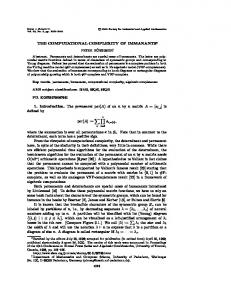
Fig. 1. An example graph and its two 3-node failure states.

A special case of the K-terminal problem is the following K-terminal node connectedness problem: In this model, edges do not fail, but the nodes that are not in a specified subset K do fail with known probabilities. The K-terminal node connectedness reliability of a graph G is then the probability that the surviving nodes of G induce a subgraph in which all nodes of K lie in a single component. This problem also was shown to be NP-hard for general graphs and it remains so even for chordal graphs and comparability graphs [1]. In this paper, we are concerned with the following reliability problem: The edges of the graph are perfectly reliable but the nodes fail independently of each other. The network is considered to be in an operational state if the surviving nodes induce a connected subgraph of G. The residual node connectedness reliability of a graph G, denoted R(G), is the probability that the graph induced by the surviving nodes is nonempty and connected. We first note that this problem is not a special case of the previous one; indeed it is very different from the K-terminal reliability problem. The K-terminal problem constitutes a hierarchical system while the residual connectedness problem does not. Specifically, let E be a finite set and P(E) be the power set of E. A system (E, Ω) consists of E and a collection of operating states Ω ⊂ P(E). A hierarchical system (E, Ω) is one where Ω is closed upward with respect to set inclusion, i.e., a superset of an operating state is again an operating state. We say that the system is operational if the collection of operating components is an operating state of the system. Assuming a probability distribution Pr on P(E), the reliability of the system is just Pr(Ω). It is easily seen that the K-terminal model and its special case described above are hierarchical. The residual node connectedness model is not hierarchical since a supergraph of a connected graph may be disconnected, as illustrated in Fig. 1. Moreover, it seems that the computational aspects of the two problems are also very different. For example, computing RK (Kn ) for a complete graph on n nodes, in which the edge failure probabilities are not necessarily equal, is clearly NP-hard. On the Q contrary, computing R(Kn ) is trivial because R(Kn ) = 1 − ρ(i), where ρ(i) is the failure probability of node i. Q Yet another example is the case where the given graph G is a tree. While RK (G) = (1 − ρ(i)), where ρ(i) is the failure probability of edge i, computation of R(G) requires a nontrivial, though linear time, algorithm; see [3]

3 for details. In this paper we show that computing the residual connectedness reliability is NP-hard. Indeed, we show that the problem remains hard even for split graphs and planar and bipartite graphs. 2. Complexity of the residual node connectedness problem. Let G be an undirected graph with e perfectly reliable edges and n nodes which fail independently and with equal probabilities ρ. Let Sk (G) be the number of connected node induced subgraphs of G with k nodes. Then the residual node connectedness reliability R(G) may be written as n X R(G, ρ) = Sk (G)ρn−k (1 − ρ)k . k=0

Pn We first show that the problem of computing S(G) = k=0 Sk (G) is #P-complete for split graphs G. Since R(G, 1/2) = S(G)/2n for ρ = 1/2, it follows that computing R(G) for split graphs is NP-hard. An undirected graph G = hV, Ei is a split graph if there is a partition V = I ∪ C such that the nodes of I form an independent set of G while the nodes of C induce a clique in G. Theorem 1. It is #P-complete to compute S(G) for split graphs G. Proof. It is clear that computing S(G) is in #P. For hardness we show that the problem of counting the number of satisfying truth assignments of a monotone boolean formula in 2-conjunctive normal form is polynomial-time Turing reducible to computing S(G) for a suitably defined graph G. For the hardness of monotone 2-SAT, see [7]. Consider a boolean formula Φ in 2-CNF with variables x1 , · · · , xr and clauses c1 , · · · , cs . We may safely assume that every variable occurs in at least one clause. For any t ≥ 1 we now define a graph Gt associated with formula Φ as follows: Gt has vertices xi , i = 1, · · · , r, and cτj , j = 1, · · · , s, τ = 1, · · · , t corresponding to the variables and clauses of Φ, respectively. Each clause is represented t times. There is an edge from xi to cτj (for all τ ≤ t) if and only if variable xi occurs in clause cj . Furthermore, there are edges that make X = {x1 , · · · , xr} into a clique. Thus Gt is a split graph, see Fig. 2. Let us define the weight of a truth assignment α : X → {0, 1} to be w(α) := number of clauses of Φ satisfied by α. Also let Tk be the number of satisfying truth assignments of weight k, k = 0, · · · , s. Note that there is a natural class Cα of connected subgraphs associated with every truth assignment α of weight at least 1. A connected subgraph C in Cα has the form C = Xα ∪ S, where Xα := { x ∈ X α(x) = 1 } and S is an arbitrary subset of { cτj α satisfies clause j, τ = 1, · · · , t }. For the sake of completeness define C∅ := { {cτj } j = 1, · · · , s, τ = 1, · · · , t }, where ∅ denotes the trivial truth assignment of weight 0. Observe that all these classes are disjoint. Furthermore, Cα has cardinality (2t )w(α) for all α 6= ∅. It is easy to verify that every connected subgraph of Gt belongs to one of these classes. Consequently, we have X S(Gt ) = st + Tk (2t )k . 1≤k≤s

4

Fig. 2. The split graph Gt constructed in the proof of theorem 2.1.

Plainly, the right-hand side is essentially a polynomial of degree s with coefficients Tk . By choosing s + 1 values of t we can thus compute the coefficients in polynomial-time, see [7]. But Ts is the number of satisfying truth assignments of Φ and we are done. In the following hardness argument for planar graphs we will use the fact that it is possible to protect certain vertices against deletion provided the total number of deleted vertices is small. More precisely, let G = hV, Ei be an arbitrary graph on n points and P ⊂ V a collection of nodes to be protected. Define a new graph G(P ) as follows: for every vertex v of G add n + 1 new vertices v1 , · · · , vn+1 and edges {v, vi }, i = 1, · · · , n + 1. Thus the new vertices vi are endpoints in G(P ). Letting p := |P |(n + 1) the cardinality of G(P ) is n0 = n + p. Now define Sk (G; P ) := number of connected induced subgraphs of G on k points containing P . We claim that for all k ≤ n (1)

Sn0 −k (G(P )) =

X p  Sn−i (G; P ). k−i i≤k

To see this, first note that since k ≤ n it is impossible to delete all the endpoints attached to any vertex in P . Hence the deletion of a vertex in P produces isolated vertices. But then any connected subset C of G(P ) of cardinality n0 − k contains all protected vertices and our claim follows. Note that G(P ) is planar and bipartite whenever G is. Substituting k = 0, · · · , n in (1) we obtain a system of n + 1 linear equations. Note that the system is in triangular form and each equation has leading coefficient 1. Hence we can compute the values Sn−i (G; P ), for k = 0, · · · , n from Sn0 −k (G(P )) in polynomial time.

5 As in Lichtenstein [4], define a graph gr(Φ) associated with formula Φ in 3-CNF as follows. For each boolean variable x of Φ there is a vertex v(x) in gr(Φ). As we will see below, v(x) represents the variable x as well as the negated variable x ¯. Similarly, each clause c of Φ is represented by a vertex v(c). There is an edge from v(x) to v(c) in gr(Φ) if and only if one of the literals x or x ¯ occurs in clause c. Furthermore, gr(Φ) contains an additional cycle through the vertices corresponding to variables. The formula Φ is planar if and only if gr(Φ) is planar. It is shown in [4] that for every boolean formula Φ there exists a planar boolean formula Φ0 which can be constructed from Φ in polynomial-time that is satisfiable if and only if Φ is satisfiable. It is easy to verify that Lichtenstein’s transformation is parsimonious, i.e., it preserves the number of satisfying truth assignments. For the hardness of 3-SAT, see [7]. Thus we have the following lemma. Lemma 2. Counting the number of satisfying truth assignments of planar boolean formulae in 3-conjunctive normal form is #P-complete. We will refer to this problem as P-3-SAT. Let us define n X ˜ S(G) := Sk (G) · 2kn . k=0

˜ S(G) will be used in the next theorem as a technical device to show that it is #Pcomplete to compute the sequence S0 (G), · · · , Sn (G). ˜ Theorem 3. It is #P-complete to compute S(G) even if G is required to be planar and bipartite. ˜ Proof. It is clear that computing S(G) is in #P. By Lemma 2.2 it suffices to ˜ show that P-3-SAT is polynomial-time Turing reducible to computing S(G) where G is required to be planar and bipartite. So assume Φ is a planar boolean formula Φ in 3-conjunctive normal form with, say, r variables and s clauses. Denote by X the set of variables of Φ and by C the set of clauses. For any variable P x, let µ(x) be the number of occurrences of the literals x and x ¯ in Φ and set m := x∈X µ(x). Now consider the planar graph H = gr(Φ). It is safe to assume that we have a planar embedding of H. In particular, we assume an appropriate cyclic ordering of the edges in H incident upon v(x) for all the vertices v(z) corresponding to boolean variables z in H. We will modify H in a number of steps that preserve planarity and produce a new graph G. First we replace all the vertices v(x), x ∈ X, by crossover boxes. We give a detailed description of one such box B, see also Fig. 3. Pick vertex v(x) ∈ X and let µ = µ(x). The crossover box B is a “broken” wheel of size 4µ; more precisely, B has vertices v(x0 ), · · · , v(x2µ−1 ), u, u0 , · · · , u2µ−1 and edges {v(xj ), u}, {v(xj ), uj }

and {uj , v(xj+1 )}

for all j < 2µ (here, as in the following, indices are supposed to be computed modulo some appropriate number). Thus u is the hub of the wheel, the vertices of the form v(xj ) and uj alternate on the perimeter, and the hub is connected to the v(xj ) vertices only.

6

Fig. 3. A crossover box in the graph representing formula Φ0 . The corresponding variable has multiplicity 3. The full nodes are protected.

Next we replace the edges {v(x), v(c)}, x ∈ X, c ∈ C, in H by new edges {v(xj ), v(c)} as prescribed by the planar embedding. We adopt the convention that j is chosen even whenever the occurrence of x in clause c is positive and odd otherwise. Furthermore, every vertex v(xj ) is used at most once. The last step is to connect the crossover boxes according to the cycle on X in H. To this end the old edges of the form {v(x), v(y)}, x, y ∈ X, are replaced by {v(xj ), uxy }, {v(xj+1 ), uxy }, {uxy , v(yj 0 )}, and {uxy , v(yj 0 +1 )}, where the uxy are new vertices and j and j 0 are chosen according to the planar embedding. A moment’s thought shows that the resulting graph G on n = s+2r +4m vertices is still planar. Furthermore, all cycles in G are necessarily of even length; hence G is in addition bipartite. We now show how to interpret the changes in the graph in terms of the boolean formula. For each x ∈ X, introduce new boolean variables x0 , · · · , x2µ(x)−1 . Then replace each occurrence of x in clause c by x2j whenever {v(x2j ), v(c)} is an edge in G. Similarly, each occurrence of x ¯ is replaced by some x2j+1 , 0 ≤ j < µ(x). Call the resulting boolean formula Φ0 . Note that Φ0 will in general fail to be planar. Also define a formula ^ Φ00 = xj ∨ xj+1 . x∈X 0≤j