THE CONNECTION BETWEEN THE COMPLEX-STEP ... - CiteSeerX

AIAA-2001-0921

THE CONNECTION BETWEEN THE COMPLEX-STEP DERIVATIVE APPROXIMATION AND ALGORITHMIC DIFFERENTIATION Joaquim R. R. A. Martins, ∗ Peter Sturdza, † and Juan J. Alonso Department of Aeronautics and Astronautics Stanford University, Stanford, CA

Abstract

‡

have been described by the authors.1, 4 In this paper we present further research on the complex-step derivative approximation, starting with some of the problems that we have found in the original implementation. In the process of solving these problems, we realized that the complexstep method could be improved, leading to a form of algorithmic differentiation. Algorithmic differentiation — also known as computational differentiation or automatic differentiation — is a well known method based on the systematic application of the differentiation chain rule to computer programs.5 The first objective of this paper is to show how the complex-step derivative approximation is related to algorithmic differentiation, further contributing to the understanding of this relatively new method. On the implementation side, we will continue to focus on automatic implementations, discussing the tradeoffs between complex step and algorithmic differentiation for the cases of Fortran and C/C++. Finally, computational results corresponding to these two programming languages will be presented.

This paper presents improvements to the complexstep derivative approximation method which increase its accuracy and robustness. These improvements unveil the connection to algorithmic differentiation theory. The choice between these two methods then hinges on a trade-off between ease of implementation and execution efficiency. Automatic implementations for Fortran and C/C++ are presented and their relative merits are discussed. These new methods were successfully implemented in two very large multidisciplinary programs and the resulting sensitivities are shown to be as accurate as the analyses. Accuracy and ease of implementation make these tools very attractive options for sensitivity analysis.

Introduction Sensitivity analysis is an important field of engineering research. One of its main applications is for design optimization methods that use gradient-based optimizers. The calculation of sensitivity information is usually the costliest step in the optimization cycle and the optimization process often fails due to inaccurate sensitivity information. The complex-step derivative approximation is a method for estimating sensitivities that has been shown to have a relatively easy implementation while yielding very accurate results.1 The potential of this technique has been recognized and it has been used in CFD sensitivity analysis by Anderson2 and in an MDO environment by Newman.3 The details and automatic implementation of this method

The Connection Complex-Step Method Basics Finite-differencing formulae are common for estimating derivatives. These formulae may be derived by truncating a Taylor series expansion about a given point x. When estimating sensitivities using these formulae we are faced with the “step size dilemma”, i.e. the desire to choose a small step size to minimize truncation error while avoiding the use of a step so small that errors due to subtractive cancellation become dominant. The complex-step derivative approximation is an equally simple first derivative estimate for real functions and may be obtained using complex calculus. If f is a real function of real variables and it is analytic, we can expand it in a Taylor series about a

∗ Graduate

Student, AIAA Student Member Student, Not an AIAA Member ‡ Assistant Professor, AIAA Member † Graduate

c Copyright °2001 by the authors. Published by the American Institute of Aeronautics and Astronautics, Inc., with permission.

1 American Institute of Aeronautics and Astronautics

real point x using an imaginary step ih. Solving this series for the first derivative yields the following approximation: ∂f Im [f (x + ih)] f 000 (x) = + h2 + ... ∂x h 3!

to use the complex-step method may be vulnerable to this weakness. Another potential problem may arise when the following complex definition of sine is used,

(1) sin(z) =

The result is an O(h2 ) estimate of the derivative of f which is not subject to subtractive cancellation error, since it does not involve a difference operation. This constitutes a tremendous advantage over the finite-difference approach. For more details on the theory and implementation of this method, the reader is encouraged to consult previously published work.1

(4)

If z = x + ih, then the imaginary part of the above equation is Im [sin(x + ih)] = cos(x)

eh − e−h . 2

(5)

This term becomes a problem when h is very small since subtraction of two very similar numbers — eh and e−h — leads to subtractive cancellation. This formula is not used in the numeric libraries used by the authors for the calculation of sine and cosine, but it may appear in the definitions of tangent and hyperbolic tangent whose complex definitions must often be supplied by the user. Rather than using the definition given in Equation (4), the following expression is preferred:

Improving the Complex-Step Method When using the complex-step derivative approximation, in order to effectively eliminate truncation errors, it is typical to use a step that is many orders of magnitude smaller than the real part of the calculation. For most operations, having real and complex parts that differ by many orders of magnitude does not pose a problem, as the real and imaginary parts effectively remain separate. With 64 bit floating point precision, for example, a complex step of 10−20 results in no truncation errors if the real part of the computation is of order one. However, there are some complex functions where a small imaginary part may vanish. Consider, for example, the definition of the inverse sine function as used in the previous implementation:1 h i p arcsin(z) = −i log iz + 1 − z 2 . (2)

sin(x + ih) = sin(x) cosh(h) + i cos(x) sinh(h). (6) Note that this expression, for small h, simplifies to sin(x + ih) ≈ sin(x) + ih cos(x).

(7)

The real part reduces to the function itself, and the imaginary part to its derivative multiplied by the step size. The application of this approach to the inverse sine function definition expressed in Equation (2) can yield an excellent replacement for that equation. By setting z = x + ih and applying the approximation for small h, we obtain

This function does not maintain accurate derivatives if the complex step is too small because it mixes the imaginary and real parts of the numbers during its computation. If z = x + ih where x = O(1) and h = O(10−20 ), then in the following operation, iz + z = (x − h) + i (x + h) ,

eiz − e−iz . 2i

arcsin(x + ih) ≡ arcsin(x) + i √

h . 1 − x2

(8)

This is a much improved definition of the inverse sine for the purpose of calculating the function sensitivity. Not only is the original difficulty with small step sizes solved, but truncation error is eliminated entirely. The real part is the inverse sine function itself, and the imaginary part, when divided by h, is the exact derivative of the function for any value of h. It is obvious from a Taylor series expansion that such an improved function definition can be found for any analytic complex function, f , by linearizing about h = 0, i.e.,

(3)

h disappears when using finite-precision arithmetic and the the derivative information is lost. Similarly, in Equation (2), iz is added to a term with the same magnitude as z. If small enough, the imaginary part, which carries the derivative information, disappears when using finite precision arithmetic resulting in a value of zero for the derivative. Even though such an operation that exchanges real and imaginary parts would not appear explicitly in a real-valued code, it may be inadvertently introduced in the definition of complex functions. Therefore, real arithmetic codes that have been modified

f (x + ih) ≡ f (x) + ih

2 American Institute of Aeronautics and Astronautics

∂f (x) . ∂x

(9)

Algorithmic ∆x1 = 1 ∆x2 = 0 f = x1 x2 ∆f = x1 ∆x2 + x2 ∆x1

The end result is a sensitivity calculation method that is essentially equivalent to algorithmic differentiation. This means that the complex-step method, as the step size is reduced, converges to a form of algorithmic differentiation that is very simple to implement for programming languages with intrinsic complex variable types that permit function overloading.

df /dx1 = ∆f

Complex-Step h1 = 10−20 h2 = 0 f = (x1 + ih1 )(x2 + ih2 ) f = x1 x2 − h1 h2 +i(x1 h2 + x2 h1 ) df /dx1 = Im f /h

Table 1: The differentiation of the multiplication operation f = x1 x2 with respect to x1 using algorithmic differentiation and the complex-step derivative approximation.

Algorithmic Differentiation As mentioned previously, algorithmic differentiation has been in use for a long time.5, 6 The method is based on the application of the chain rule of differentiation to each operation in the program flow. For each intermediate variable in the algorithm, a variation due to one input variable is carried through. As a simple example, suppose we want to differentiate the multiplication operation, f = x1 x2 , with respect to x1 . Table 1 compares how the differentiation would be performed using either algorithmic differentiation or the complex-step method. As we can see, algorithmic differentiation stores the derivative value in a separate set of variables while the complex step carries the derivative information in the imaginary part of the variables. It is shown that in this case, the complex-step method performs one extra operation — the calculation of the term h1 h2 — which, for the purposes of calculating the derivative is superfluous. The complex-step method will nearly always include these superfluous computations (which can also be identified in Equation (6).) The extra computations correspond to the higher order terms in the Taylor series expansion of Equation (1). Although this example involves only one operation, both methods work for an algorithm involving an arbitrary sequence of operations by propagating the variation of one input forward throughout the code. This means that in order to calculate n derivatives, the differentiated code must be executed n times. This particular form of algorithmic differentiation is called the forward mode. It calculates the derivatives of all the outputs with respect to one input. The other mode — the reverse mode 5 — has no equivalent in the complex-step method. When using the reverse mode, the code is executed forwards and then backwards to calculate derivatives of one output with respect to n inputs. The total number of operations is independent of n, but the memory requirements may be prohibitive, especially for the case of large iterative algorithms. Since the use of the complex-step method has only

recently become widespread, there are some issues that seem unresolved. However, now that this connection to algorithmic differentiation has been established, we can look at the extensive research that has been done on the subject of algorithmic differentiation for some answers. Important issues include how to treat singularities,7 differentiability problems due to if statements,8 and the convergence of iterative solvers,9, 10 all of which have been addressed by the algorithmic differentiation research community. The singularity issue — i.e. what to do when the derivative is infinite — is handled automatically by the complex-step method, at the expense √ of some accuracy. For example, the computation of x + ih √ 1 differs substantially from x + ih 2√ as x vanishes, x but this has not produced noticeable errors in the large algorithms that we tested. Regarding the issue of if statements, in rare circumstances, modification of the original algorithm is necessary as its differentiability may be compromised by piecewise function definitions. Finally, concerning convergence of iterative codes, the experience of the authors has been that in all cases the imaginary part converges at a rate similar to the real part, although somewhat lagged. Furthermore, for engineering applications where the iterative process converges to a differentiable function, it is our experience that the derivative also converges to the correct result.

Implementations The implementation of any of the derivative calculation methods, for practical purposes, should be as automated as possible. Changing the source code manually is not only an extremely tedious task, but is also likely to result in the introduction of coding errors in the program.

3 American Institute of Aeronautics and Astronautics

There are two main possibilities for implementing algorithmic differentiation: by source code transformation or by using derived datatypes and operator overloading. To implement algorithmic differentiation by source transformation, the whole code must be processed with a parser and all the derivative calculations are introduced as extra lines of code. The resulting extended code is greatly enlarged and it becomes practically unreadable. This fact constitutes an implementation disadvantage as it becomes impractical to debug this new extended code. One has to work with the original source, and every time it is changed (or if different derivatives are desired) one must rerun the parser before compiling the new version. In order to use derived types, we need languages that support this feature, such as Fortran 90 or C++. A new type of structure must be created that contains both the value and its derivative. All the existing operators must then be re-defined for the new type. The new operator would have exactly the same behaviour as before for the value part of the new type, but use the derivative of the operator to calculate the derivative portion. This results in a very elegant implementation since very few changes are required in the original code. In the following section, implementations of these methods will be described in detail for Fortran and C/C++. Some notes for other programming languages will also be included.

with a multitude of subroutines, this approach may be time consuming and prone to errors. The automatic Fortran differentiation tool presented in this paper is an improved version of the complex-step method published previously.1 It is composed of a a Python script that makes the necessary changes to the source code and Fortran 90 module that contains overloaded function definitions. The Python script has been enhanced by adding support for a wider range of platforms and compilers as well as support for MPI based parallel implementations. Further flexibiliy was added to the script by addressing file input and output issues. The new version of the complexify module has been improved by using the new function definitons discussed in the previous section, i.e., definitions that use the original real function for the real part and the derivative of the function multiplied by h for the imaginary part, rather than the complex function definition. These new definitions only apply to functions that are not defined for complex arguments in standard Fortran, such as tangent, inverse trignometric functions and hyperbolic functions. The reason for not using these improved definitions for all functions is that Fortran 90 does not permit the redefinition of functions that already exist. The way around this restriction would be to create a new type of variable, thus allowing the use of our own function definitions. This is the approach adopted by the algorithmic differentiation methods that use derived datatypes. The drawbacks with this approach are that there are far more changes required to the original source code and it is no longer compatible with some old Fortran constructs. This tool for implementing the complex-step method represents, in our opinion, a good compromise between ease of implementation and algorithm efficiency. While pure algorithmic differentiation is numerically more efficient, the method used in this paper requires far fewer changes to the original source code resulting in improved maintainability. Furthermore, practically all the changes are performed automatically by the use of the script. All the necessary files, together with detailed instructions are available on the first author’s webpage.4

Fortran Many tools for automatic algorithmic differentiation of Fortran programs by source transformation already exist. Some of these are ADIFOR, TAMC, DAFOR, GRESS, Odysse and PADRE2.11 As explained above, extending the original source code is a method that greatly compromises the code’s maintainability. There are also tools for automatic algorithmic differentiation of Fortran programs by using derived datatypes and operator overloading such as AD01, ADOL-F, IMAS and OPTIMA90.11 They have been extensively developed and provide the user a lot of functionality. However, all of these require the user to make a series of changes to the source code by hand. These include selective changes to variable type declarations, the addition of use statements, as well as the modification of input, output and variable initialization statements. When dealing with a large program

C/C++ The C/C++ implementations of the complex-step method and algorithmic differentiation are much more straightforward than the Fortran implementations. Two different C/C++ implementations are

4 American Institute of Aeronautics and Astronautics

Platform Compiler Executable size (KB) Real Complex Surreal

Sun Ultra1 143MHz g++ 2.95.2 1680 3.84 11.99 (3.1) 6.91 (1.8)

Sun Ultra60 358MHz CC SunWorks 5.0 1400 1.95 9.38 (4.8) 4.73 (2.4)

Intel Celeron 429MHz g++ 2.91.66 1032 1.07 3.83 (3.6) 2.31 (2.2)

SGI Octane IP30 195MHz MIPSpro 7.30 846 1.21 2.68 (2.2) 1.91 (1.6)

Table 2: Run times (in seconds) for a boundary layer solution with no derivatives; with derivatives via the complex-step method; and with derivatives using an algorithmic differentiation method. presented and used in this paper and are available on the web.4 The first method is analogous to the Fortran implementation, i.e., it uses complex variables and overloaded complex functions and operators. An include file, complexify.h, defines a new variable type called cmplx and all the functions that are necessary in the implementation of the complex-step method. The inclusion of this file and the replacement of double or float declarations with cmplx is nearly all that is required. The remaining work involves dealing with input and output routines. The usual casting of the inputs to cmplx and printing of the outputs using the real() and imag() functions works well. For ASCII files or terminal input and output, the use of the C++ iostream library is also possible. In this case, the “À” operator will automatically read in a real number and properly cast it to cmplx, or read in a complex number in the Fortran parenthesis format, e.g., “(2.3,1.e-20)”. The “¿” operator will output in the parenthesis format. The second method is a version of algorithmic differentiation that is basically a realization of Equation (9). It can be implemented by including a file called derivify.h and by replacing declarations of double with declarations of surreal. The derivify.h file redefines all relational operators, the basic arithmetic formulae, trigonometric functions, and other formulae in the math library when applied to the surreal variables. These variables contain “value” and “derivative” parts analogous to the real and imaginary parts of complex variables. It works just as the complex step version does, except that the step size may be set to 1 since there is no truncation error. One feature available to the C++ programmer is worth mentioning: templates. Templates make it possible to write source code that is independent of variable type declarations. This approach in-

volves considerable work with complicated syntax in function declarations and requires at least a bit of object-oriented programming. There is no need, however, to modify the function bodies themselves or to change the flow of execution, even for pure C programs. The distinct advantage is that the variable types can be decided at run time, so the very same executable can run either the real-valued, the complex step or the algorithmic differentiation version. This considerably simplifies version control and debugging since updating or debugging one version of the code updates and debugs the others — the source code is literally the same for all three versions of the program. An execution speed comparison of the complex step and pure algorithmic differentiation method on a finite-difference boundary layer code is shown in Table 2. The rows labeled “Real,” “Complex” and “Surreal” contain execution times in seconds, and, in parentheses, the ratios of the latter two methods to the real-valued execution times. This program uses C++ templates to implement the three methods, so the size of the executable can increase considerably. When comparing to the real-valued code, the executables here are 5 to 7 times larger. However, there was no time or memory penalty due to the use of templates. The basic result is that, as is often stated, the complex variable version of the program takes about three times longer to run than the real-valued version, and the algorithmically differentiated code takes about twice as long as the real-valued program. Interestingly, the SGI platform is much more efficient at computing derivatives than the other systems, either due to a better compiler, its 64 bit hardware architecture, or both. It should be noted that there are much more sophisticated algorithmic differentiation packages available for C/C++.11 The one presented here is

5 American Institute of Aeronautics and Astronautics

meant as a simple improvement to the complex-step method that is equally easy to implement. Other packages include ADIC,12 an implementation mirroring ADIFOR, and ADOL-C,13 a free package that uses operator overloading and can operate in forward and reverse modes as well as compute higher order derivatives.

0

10

C D ∂ CD / ∂ M∞

−5

Relative Error, ε

10

Other Programming Languages In addition to the Fortran and C/C++ implementations described above, some work was done with other programming languages. The complex-step method works well under Matlab with practically no changes to the user’s source code.1 A simple implementation of the complex-step method for Python was also developed for the purposes of this paper. In order to do this, one must import cmath, a standard module for complex arithmetic. Then, just as in Fortran 77 or C, functions such as c abs, c atan2 and c max must be defined. Since Python supports operator overloading, a more elegant algorithmic differentiation method similar to that used in C++ also seems possible. In general, algorithmic differentiation can be implemented in any programming language that supports derived datatypes and operator overloading. For languages that do not have these features, the complex-step method can be used wherever complex arithmetic is supported.

−10

10

−15

10

50

100

150

200

250 300 Iterations

350

400

450

500

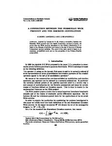
Figure 1: Convergence of CD and ∂CD /∂M∞ for the |f −f | 2D flow solver.; ε = |frefref| . drag coefficient converges to the algorithm’s precision, which is almost machine zero. The sensitivity is shown to lag slightly in the convergence. This is expected, since the calculation of the sensitivity of a given quantity is dependent on the value of that same quantity. After the drag coefficient result achieves the algorithm’s precison, the sensitivity catches up after about 20 additional iterations.

0

10

Complex−Step Finite−difference

Results −5

Relative Error, ε

Two-Dimensional Flow Solver The automatic implementation of the complex-step method for FLO82 — a two-dimensional finite volume solver for the Euler equations — has been decribed in previous work.1 Although the results that were presented therein are correct, they did not achieve the full working precision of the algorithm because of an error in the compilation. Therefore, we will show results from the same solver that were obtained using the latest implementation of the complex-step method. Since the flow solver is an iterative algorithm, it is useful to compare the convergence of a given result with that of its derivative, which is contained in its complex part. This comparison is shown in Figure 1 for the drag coefficient and its derivative with respect to the freestream Mach number. The

10

−10

10

−15

10

−10

10

−20

10 Step Size, h

−30

10

Figure 2: Sensitivity estimate errors for ∂CD /∂M∞ given by finite-difference and the complex step for |f −f | decreasing step size; ε = |frefref| . The next plot, Figure 2, shows a comparison between the estimates of ∂CD /∂M∞ given by both the complex-step and the forward-difference methods for

6 American Institute of Aeronautics and Astronautics

namic analysis is performed by Reuther et al.’s SYN107-MB15 — a multiblock Euler flow solver — which also calculates the sensitivity of the drag and other aerodynamic quantities with respect to wing geometry perturbations using an adjoint method. These perturbations are the shape design variables and consist of “bump” functions distributed on the top and bottom surfaces of the wing.15 The wing structure is modeled with FESMEH,16 a finite element solver which includes the following wing structural components: wing skins, spars and ribs. In addition to solving for displacements and stresses, the structural solver is able to calculate the derivatives of these quantities with respect to element dimensions analytically. The coupling of the aerodynamic and structural analysis codes has previously been developed by the authors and uses a consistent and conservative scheme.14 The aero-structural model and a sample solution are shown in Figure 3. The internal structure of the wing and a slice of the 3D CFD grid are shown.

various step sizes. The forward-difference estimate initially improves since the O(h) truncation error decreases with step size. However, as the step is reduced below a value of about 10−10 , subtractive cancellation errors become an issue and the estimates become unreliable. When the interval h is so small that no difference exists in the output — for steps smaller than 10−17 — the finite-difference estimates eventually yield zero. The complex-step estimate improves quadratically as the step size is decreased. The estimate is practically insensitive to variations of step size below an h of the order of 10−10 , value for which the estimate achieves the accuracy of the flow solver. Although the complex step size can be made extremely small, there is a lower limit (h = 10−321 ) below which underflow starts to occur and the estimate results in NaN. When comparing the best accuracy of these approaches, we see that finite-differencing only achieves a fraction of the accuracy of the complexstep approximation. Three-Dimensional Aero-Structural Solver

CD ∂ CD / ∂ b1

0

10

The tools that we have developed to implement the complex-step method automatically were also tested on a much larger application: a high-fidelity aerostructural solver that is part of an MDO framework which was created to solve wing design optimization problems.14 Since an analytic method for calculating sensitivities is being developed for this analysis code, the complex-step method will be an extremely useful reference for validation.

Reference Error, ε

−2

10

−4

10

−6

10

−8

10

100

200

300

400 Iterations

500

600

700

800

Figure 4: Convergence of CD and ∂CD /∂b1 for the |f −f | 3D aero-structural solver; ε = |frefref| . To validate the complex-step results for this solver, we chose the derivative of the drag coefficient to the shape perturbations, accounting for the structural displacements. There is a three by three grid of perturbations on each of the wing’s surfaces making up for a total of 18 design variables. A plot of the convergence of the drag coefficient is also shown for this case (see Figure 4), together with the convergence of the sensitivity corresponding to the first shape design variable, b1 . As with the case of the two-dimensional flow solver, the derivative converges at the same rate as

Figure 3: Aero-structural model and solution of a transonic jet configuration, showing a slice of the grid and the wing’s internal structure. Within the aero-structural solver, the aerody7

American Institute of Aeronautics and Astronautics

the coefficient and it lags slightly, taking about 100 additional iterations to achieve the maximum precision. The maximum precision of the derivative is observed to be slightly lower than the precision of the coefficient. When looking at the number of digits that are converged, the coefficient consistently converged to six digits, while the derivative converged to five or six digits. This might be explained by the increased round-off errors of complex arithmetic,17 which does not affect the real part when such small step sizes are used.

Complex−Step, h = 1×10−20 −2 Finite−Difference, h = 1×10

0.15

∂ CD / ∂ bi

0.1

0.05

0

−0.05

0

10

2

Complex−Step Finite−difference

−1

10

6

8 10 12 Shape variable, i

14

16

18

Figure 6: Comparison of the estimates for the shape sensitivities of the drag coefficient, ∂CD /∂bi .

−2

10 Relative Error, ε

4

−3

10

Supersonic Viscous/Inviscid Solver −4

10

The following example illustrates how the complexstep method can be applied to an analysis from which it is very difficult to extract accurate finite difference gradients. It is a complicated code that uses input and output file manipulations to combine five computer programs including an iterative Euler solver and boundary layer solutions featuring transition prediction. This code was developed for supporting design work of the supersonic Natural Laminar Flow aircraft concept.18 In this framework, Python is used as the glue that joins the many programs that constitute the function analysis with an optimizer that requires values and derivatives of the objective and constraints. Gradients are computed with the complex-step method and with algorithmic differentiation in the Fortran, C++ and Python programming languages. The sequence of calculations for each function evaluation is as follows:

−5

10

−6

10

−5

−10

10

10

−15

10

Step Size, h

Figure 5: Sensitivity estimate errors for ∂CD /∂b1 given by finite-difference and the complex step for |f −f | different step sizes; ε = |frefref| . Figure 5 shows a plot analogous that of Figure 2. In this case the finite-difference result has an acceptable precision for only one step size (h = 10−2 ). Again, the complex-step method yields accurate results for step sizes ranging from h = 10−2 to h = 10−200 . The results corresponding to the complete shape sensitivity vector are shown in Figure 6. Although many different sets of finite-difference results were obtained, only the best set is plotted here. The plot shows no discernible difference between the two sets of results. Again, we would like to emphasize that while there was considerable effort involved in obtaining reasonable finite-difference results by trying different step sizes, no such studies were necessary with the complex-step method.

• The Python wrapper program is given a list of design variables by the optimizer. It then begins by computing, using complex variables, a geometry description for the grid generator. • CH GRID, written by D. Saunders and J. Reuther at NASA Ames, automatically generates a 3D grid for either a wing alone or a wingbody. It is a Fortran 90 program which was complexified with the script described in this paper. • CFL3D19 provides the supersonic Euler flow so8

American Institute of Aeronautics and Astronautics

2

10

Finite Difference Complex−Step 0

Relative Error, ε

10

−2

10

−4

10

−6

10

−8

10

0

10

−5

10

−10

10 Step Size, h

−15

10

−20

10

Figure 8: Convergence of gradients as step size is |f −f | decreased. ε = |frefref| . Figure 7: Trapezoidal wing with 5% thick biconvex airfoils, 32◦ leading edge sweep, 22.5 ft root chord, 5.45 ft tip chord and 18.94 ft semispan.

The results presented here are gradients of the skin-friction drag coefficient with respect to the root chord of the trapezoidal wing depicted in Figure 7 at Mach 2.0, 40,000 ft and 4◦ angle of attack. The other design variables are the tip chord, the root and tip thickness to chord ratios, the leading edge sweep and the tip twist. Twist and thickness vary linearly spanwise, and the area is held constant. Therefore, when the root chord varies, the trailing edge sweep and wingspan change. A comparison of finite central difference results with the complex-step gradients is shown in Figures 8-11. The first one, computed with a laminar boundary layer, shows the rather poor quality finite difference gradients of this analysis. There are several properties of this analysis that make it difficult to extract useful finite difference data. The most obvious is transition. It is difficult to truly smooth the movement of the transition front when transition prediction is computed on a discretized domain. Since transition has such a large effect on skin friction, this difficulty is expected to adversely affect finite difference gradients of drag. Additionally, the discretization of the boundary layer by computing it along 12 arcs that change curvature and location as the wing planform is perturbed is suspected to cause some noise in the laminar solution as well (these arcs, their purpose, and further details of the boundary layer solution and transition prediction are described elsewhere.18 ) A plot of the gradient itself in Figure 9 shows that finite difference and complex-step results do agree for step sizes larger than 0.001 feet. Figure 10 de-

lution. Starting with Version 6, CFL3D comes with the complex-step method already implemented. • The Euler solution is post-processed by a C++ program that was complexified following the description in this paper. • A quasi-3D boundary-layer solver18 is then executed on the wing at six spanwise stations, top and bottom, by the Python wrapper (viscousinviscid iterations are not required at the supersonic flight conditions of this NLF aircraft). It can compute laminar and turbulent boundary layers and also has the capability to predict the transition location. This boundary-layer solver uses the C++ algorithmic differentiation approach. • The Python wrapper merges the 12 boundary layer solutions to produce a three-dimensional skin-friction drag result to which it adds the inviscid drag computed by CLF3D and computes other quantities to evaluate constraints (such as wing structural weight constraints). • The above steps are repeated for each of the design and constraint variables, and then the Python wrapper passes the values and derivatives to the optimizer.

9 American Institute of Aeronautics and Astronautics

−5

−4

x 10

x 10 4.3736

Finite Difference Complex−Step

2

Function Evaluations Complex−Step Slope

4.3735 4.3734

1

4.3732

Cdf

dCdf / dCr

4.3733

0

4.3731

−1 4.373 4.3729

−2

4.3728

−3 0

10

−2

10

−4

10

−6

10 Step Size, h

−8

10

22.495

−10

22.5 Root Chord (ft)

10

22.505

Figure 10: Skin friction drag coefficient as a function of wing root chord with a laminar boundary layer.

Figure 9: Gradient of skin friction drag coefficient with respect to wing root chord computed with various step sizes (laminar boundary layer).

ing accurate and smooth gradients for analyses that accumulate substantial computational noise.

picts the drag coefficient as it varies with perturbations in root chord. The slope computed with the complex-step at 22.5 ft chord is in good agreement with the function evaluations in the vicinity. Figure 11 shows the expected noise increase for the same conditions when transition to turbulent flow is computed. The complex-step slope, however, remains very reasonable — not too far from a least squares fit of the data.

Acknowledgements The authors would like to thank Dr. James Reuther for his invaluable help, particularly with SYN107MB and the aero-structural solver. He was unfortunately demoted from the top of the first page to this section because of bureaucratic constraints.

References

Conclusions

[1] Martins, J. R. R. A., I. M. Kroo, and J. J. Alonso “An Automated Method for Sensitivity Analysis using Complex Variables” Proceedings of the 38th Aerospace Sciences Meeting, Reno, NV, January 2000. AIAA Paper 2000-0689.

New insights into the complex-step method have been presented. Solutions to several subtle problems in its implementation have been clarified, and its relationship to traditional algorithmic differentiation methods has been exposed. This enables the application of a substantial body of knowledge — that of the algorithmic differentiation community — to the complex-step method, answering many important questions. The complex-step technique may still be the easiest of any derivative calculation method to implement, particularly in legacy codes and in codes that mix programming languages. Furthermore, the resulting complexified code is no harder to debug and maintain than the original. The example implementations and their results illustrate these points clearly and put forward two excellent uses for the method: validating a more sophisticated gradient calculation scheme and provid-

[2] Anderson, W. K., J. C. Newman, D. L. Whitfield, E. J. Nielsen, “Sensitivity Analysis for the Navier-Stokes Equations on Unstructured Meshes Using Complex Variables”, AIAA Paper No. 99-3294, Proceedings of the 17th Applied Aerodynamics Conference, 28 Jun. 1999. [3] Newman, J. C. , W. K. Anderson, D. L. Whitfield, “Multidisciplinary Sensitivity Derivatives Using Complex Variables”, MSSU-COE-ERC98-08, Jul. 1998. [4] http://aero-comlab.stanford.edu/jmartins [5] Griewank, A., Evaluating Derivatives, SIAM, Philadelphia, 2000. 10

American Institute of Aeronautics and Astronautics

[13] Griewank, A., et al., “ADOL-C: A Package for the Automatic Differentiation of Algorithms Written in C/C++,” ACM TOMS, Vol. 22(2), June 199, pp. 131-167, Algorithm 755.

−3

x 10 3.0223

Function Evaluations Complex−Step Slope 3.0223

[14] Reuther, J., J. J. Alonso, J. R. R. A. Martins, and S. C. Smith, “A Coupled AeroStructural Optimization Method for Complete Aircraft Configurations”, Proceedings of the 37th Aerospace Sciences Meeting, AIAA Paper 1999-0187. Reno, NV, January 1999.

3.0222

Cd

f

3.0222 3.0222 3.0222

[15] Reuther, J., J. J. Alonso and A. Jameson, “Constrained Multipoint Aerodynamic Shape Optimization Using an Adjoint Formulation and Parallel Computers: Part I”, Journal of Aircraft, 36(1):51-60, 1999.

3.0222

22.495

22.5 Root Chord (ft)

22.505

Figure 11: Skin friction drag coefficient as a function of wing root chord with transition to turbulent flow in the boundary layer.

[16] Holden, M. E., “Aeroelastic Optimization using the Collocation Method”, PhD Thesis, Stanford, May 1999. [17] Olver, F. W. J., “Error Analysis of Complex Arithmetic”, Computational Aspects of Complex Analysis, pp. 279-292, 1983.

[6] Bischof, C., A. Carle, G. Corliss, A. Grienwank, P. Hoveland, “ADIFOR: Generating Derivative Codes from Fortran Programs”, Scientific Programming, Vol. 1, No. 1, 1992, pp. 11-29.

[18] Sturdza, P., V. M. Manning, I. M. Kroo, and R. R. Tracy, “Boundary Layer Calculations for Preliminary Design of Wings in Supersonic Flow,” AIAA Paper 99-3104, Proceedings of the 17th Applied Aerodynamics Conference, 28 June 1999.

[7] Bischof, C., G. Corliss, A. Grienwank, “ADIFOR Exception Handling”, Argonne Technical Memorandum, MCS-TM-159, 1991. [8] Beck, T. and H. Fischer, “The if-problem in automatic differentiation”, Journal of Computational and Applied Mathematics, Vol. 50, pp. 119-131, 1994.

[19] Krist, S. L., R. T. Biedron, and C. L. Rumsey, CFL3D User’s Manual (Version 5.0) NASA/TM-1998-208444, June 1998.

[9] Griewank, A., C. Bischof, “Derivative Convergence for Iterative Equation Solvers” Optimization Methods and Software, Vol. 2, pp. 321-355, 1993. [10] Beck, T., “Automatic Differentiation of iterative processes” Journal of Computational and Applied Mathematics, Vol. 50, pp. 109-118, 1994. [11] http://www.sc.rwth-aachen.de/Research /AD/subject.html [12] Bischof, C., L. Roh, A. Mauer, “ADIC – An Extensible Automatic Differentiation Tool for ANSI-C,” to appear in Software: Practice and Experience, also ANL/MCS-P626-1196 (ftp://info.mcs.anl.gov/pub/tech reports /reports/P626.ps.Z)

11 American Institute of Aeronautics and Astronautics