1 ; see e.g. Hamilton 1994 or Fuller 1996 and the references therein. The ..... Applying 5 we get after some simple algebra that. 1 l hb,1. X s=1. e i0 + s X s + k,1.
1
The Continuous-Path Block-Bootstrap
E. PAPARODITIS and D. N. POLITIS University of Cyprus and University of California, San Diego
Abstract - The situation where the available data arise from a general linear process
with a unit root is discussed. We propose a modi cation of the Block Bootstrap which generates replicates of the original data and which correctly imitates the unit root behavior and the weak dependence structure of the observed series. Validity of the proposed method for estimating the unit root distribution is shown. Research supported by NSF Grant DMS-97-03964 and by a University of Cyprus Research Grant.
1. INTRODUCTION Consider time series data fX (1); X (2); : : :; X (n)g arising from the process
X (t) = �X (t , 1) + U (t); for t = 1; 2; : : :, where X (1) = 0, � is a constant in [,1; 1], and Assumption A fU (t); t � 1g is a stochastic process satisfying U (t) =
1
X
j =0
j "(t , j )
(1)
(2)
1 where 0 = 1, 1 j =0 j j j j < 1, j =0 j 6= 0 and f"(t); t 2 ZZg is a sequence of independent identically distributed random variables with mean zero and 0 < E ("2(1)) < 1. We will be especially concerned with the nonstationary (integrated) case where � = 1. Note that if j = 0 for j > 1 we are in the case of a random walk, i.e., (2) allows for a wide range of weak dependence of the di�erenced process X (t) , X (t , 1). A number of papers in the econometrics literature has dealt with model (1); see e.g. Hamilton (1994) or Fuller (1996) and the references therein. The traditional approach so far has been based on the Dickey and Fuller (1979) pioneering work and consists of conducting a test of the null hypothesis that P
P
2
E. Paparoditis and D. N. Politis
there is a unit root; in this connection see also Phillips and Perron (1988), and Ferretti and Romo (1996). Recently however, there has been some interest in the attempt to go beyond the simple unit root test. Stock (1991) managed to develop con dence intervals for � in the equation X (t) = �X (t , 1)+ U (t) based on `local-to-unity' asymptotics. Hansen (1997) proposed the `grid-bootstrap' to adress this situation, and reports improved performance. Finally, Romano and Wolf (1998) applied the general subsampling methodology of Politis and Romano (1994) to the AR(1) model with good results; see Politis et al. (1999) for more details. In the paper at hand, we present a di�erent approach towards inference under the presence of a unit root; our approach is based on a modi cation of the Block-Bootstrap (BB) of Kunsch (1989), and |for reasons to be apparent shortly| is termed \Continuous-Path Block-Bootstrap (CBB)". To motivate the CBB, let us give an illustration demonstrating the failure of the BB under the presence of a unit root. Figure 1(a) shows a plot of (the natural logarithm of) the S&P 500 stock series index recorded annually from year 1871 to year 1988, while Figure 1(b) shows a realization of a BB pseudo replication of the S&P 500 series using block size 20. It is obvious visually that the bootstrap series is quite dissimilar to the original series, the most striking di�erence being the presence of strong discontinuities (of the `jump' type) in the bootstrap series that {not surprisingly- occur every 20 time units, i.e., where the independent bootstrap blocks join. Figure 1(c) suggests a way to x this problem by forcing the bootstrap sample path to be continuous. A simple way to do this is to shift each of the bootstrap blocks up or down with the goal of ensuring (i) the bootstrap series starts o� at the same point as the original series, and that (ii) the bootstrap sample path is continuous. Notably, the bootstrap blocks used in Figure 1(c) are the exact same blocks featuring in Figure 1(b). At least as far as visual inspection of the plot can discern, the series in Figure 1(c) could just as well have been generated by the same probability mechanism that generated the original S&P 500 series. In other words, it is plausible that a bootstrap algorithm generating series such as the one in Figure 1(c) would be successful in mimicking important features of the original process; thus, the \Continuous-Path Block-Bootstrap" of Figure 1(c) is expected to `work' in this case. Of course, the actual yearly S&P 500 data are in discrete time, and talking about continuity is -strictly speaking- inappropriate. Nevertheless, an underlying continuous-time model may always be thought to exist, and the idea of continuity of sample paths is powerful and intuitive; hence the name \ContinuousPath Block-Bootstrap" (CBB for short) for our discrete-time methodology as well. The CBB is described in detail in the next Section, and some of its key properties are proven.
3
The CBB for Nonstationary Processes
1
2
3
4
5
a
0
20
40
60
80
100
120
80
100
120
80
100
120
1
2
3
4
5
b
0
20
40
60
2
3
4
c
0
20
40
60
Figure 1: Plot of the natural logarithm of the S&P500 stock index series (a), of a BB realization (b) and of a CBB realization (c) with blocksize 20.
2. THE CONTINUOUS-PATH BLOCK-BOOTSTRAP (CBB) Before introducing the Continuous-Path Block-Bootstrap (CBB) Method we review Kunsch's (1989) Block-Bootstrap (BB). The BB algorithm is carried out conditionally on the original data fX (1); X (2); : : :; X (n)g, and thus implicitly de nes a bootstrap probability mechanism denoted by P ? that is capable of generating bootstrap pseudo-series of the type fX ?(t); t = 1; 2; : : :g.
Block-Bootstrap (BB) algorithm:
1. First chose a positive integer b(< n), and let i0; i1; : : :; ik,1 be drawn i.i.d. with distribution uniform on the set f1; 2; : : :; n , b + 1g; here we take k = [n=b], where [�] denotes the integer part, although di�erent choices for k are also possible. The BB constructs a bootstrap pseudoseries X ?(1); X ?(2); : : :; X ?(l), where l = kb, as follows. 2. For m = 0; 1; : : :; k , 1, let
X ?(mb + j ) := X (im + j , 1)
for j = 1; 2; : : :; b.
4
E. Paparoditis and D. N. Politis
The Continuous-Path Block-Bootstrap (CBB) algorithm is now de ned in the following three steps below. As before, the algorithm is carried out conditionally on the original data fX (1); X (2); : : :; X (n)g, and implicitly de nes a bootstrap probability mechanism denoted by P � that is capable of generating bootstrap pseudo-series of the type fX �(t); t = 1; 2; : : :g. In the following we denote quantities with respect to P � with an asterisk � .
Continuous-Path block-bootstrap (CBB) algorithm: 1. First calculate the centered residuals
1
n
X
U (t) = X (t) , X (t , 1) , n , 1 (X (t) , X (t , 1)) t=2 b
for t = 2; 3; : : :; n. Attention now focuses on the new variables Xe (t) de ned as follows: 8 for t = 1 < X (1) e X (t) = : X (1) + Ptj =2 Ub (j ) for t = 2; 3; : : :; n. 2. Chose a positive integer b(< n), and let i0; i1; : : :; ik,1 be drawn i.i.d. with distribution uniform on the set f1; 2; : : :; n , bg; here, we take k = [n=b] as before. The CBB constructs a bootstrap pseudo-series X �(1); : : :; X �(l), where l = kb, as follows. 3. Construction of the rst bootstrap block. Let
X �(j ) := X (1) + [Xe (i0 + j , 1) , Xe (i0)] for j = 1; : : :; b: To elaborate: X �(1) := X (1) X �(2) := X �(1) + [Xe (i0 + 1) , Xe (i0)] X �(3) := X �(1) + [Xe (i0 + 2) , Xe (i0)]
.. . � � X (b) := X (1) + [Xe (i0 + b , 1) , Xe (i0)]: 4. Construction of the (m + 1)-th bootstrap block from the m-th block for m = 1; : : :; k , 1. Let
X �(mb + j ) := X �(mb) + [Xe (im + j ) , Xe (im)]
The CBB for Nonstationary Processes
5
for j = 1; : : :; b: To elaborate:
X �(mb + 1) := X �(mb) + [Xe (im + 1) , Xe (im )] X �(mb + 2) := X �(mb) + [Xe (im + 2) , Xe (im )]
.. . X �(mb + b) := X �(mb) + [Xe (im + b) , Xe (im )]: An intuitive way to understand the CBB construction is based on the discussion regarding Figure 1(c) in the Introduction and goes as follows: (i) construct a BB pseudo-series fX �(t); t = 1; 2; : : :g based on blocks of size equal to b + 1 from the series Xe (t); (ii) shift the rst block (of size b + 1) by an amount selected such that the bootstrap series starts o� at the same point as the original series; (iii) shift the second BB block (of size b + 1) by another amount selected such that the rst observation of this new bootstrap block matches exactly the last observation of the previous bootstrap block; (iv) join the two blocks but delete the last observation of the previous bootstrap block from the bootstrap series; (v) repeat parts (iii) and (iv) until all the generated BB blocks are used up. Note that the CBB is applied to fXe (t)g and not to fX (t)g. The reason is that although the X (t) series is produced via the zero mean innovations U (t), the observed nite-sample realization of the innovations will likely have nonzero (sample) mean; this discrepancy has an important e�ect on the bootstrap distribution e�ectively leading to a random walk with drift in the bootstrap world. Fortunately, there is an easy x-up by recentering the innovations; a similar necessity for residual centering has been recommended early on even in regular linear regression |see Freedman (1981). Note that a CBB series using block size b is associated to a BB construction with block size b + 1. This phenomenon is only due to the fact that we are dealing with discrete-time processes; it would not occur in a continuous-time setting. The reason for this is our step (iv) above: although we are e�ecting the matching of the rst observation of a new bootstrap block to the last observation of the previous bootstrap block, it does not seem advisable to leave both occurrences of this common (matched) value to exist side-by-side; one of the two must be deleted as step (iv) suggests.
3. ESTIMATION OF THE UNIT ROOT DISTRIBUTION In this section the properties of the CBB in estimating the distribution of the rst order autoregressive coe�cient in the presence of a unit root are considered. Recall that based on the observations fX (1); X (2); : : :; X (n)g a
6
E. Paparoditis and D. N. Politis
common estimator of the rst order autoregressive coe�cient � in (1) is given by T X X (t)X (t , 1) t =2 �^ = X : (3) n 2 X (t , 1) The CBB version of � is given by l
t=2
X
X �(t)X �(t , 1)
�^� = t=2 l
(4)
X �2 (t , 1)
X
t=2
and the distribution of the statistic l(^�� , 1) is used to estimate the distribution of n(^� , 1) Consider rst the basic random walk case. For this case the following result can be established.
Theorem 1 Let X (t) = X (t , 1) + "(t), t = 1; 2; : : : where X (0)p= 0, "(t) � IID(0; � ) and E (" (1)) < 1. If b ! 1 as n ! 1 such that b= n ! 0 then sup P � l(^�� , 1) � x , P n(^� , 1) � x ! 0 2
4
x2R
�
�
�
�
in probability.
The asymptotic validity of the CBB for the general case where the stationary process fU (t)g satis es Assumption A is established in the following theorem which is our main result.
Theorem 2 Let X (t) = X (t , 1) + U (t), t = 1; 2; : : : where fU (t); t 2 ZZg satis es Assumption A and E (" (1)) < 1. If b ! 1 as n ! 1 such that b=pn ! 0 then sup P � l(^�� , 1) � x , P n(^� , 1) � x ! 0 4
x2R
�
�
�
�
in probability.
It is noteworthy that, under the assumptions of Theorem 2, the asymptotic distribution of �^ has a complicated form, depending on many unknown
7
The CBB for Nonstationary Processes
parameters such as the in nite sum 1 j =0 j ; see Hamilton (1994) or Fuller (1996). The CBB e�ortlessly achieves the required distribution estimation, and provides an attractive alternative as compared to the asymptotic distriP bution with estimated parameters. Notably, estimation of the sum 1 j =0 j is tantamount to estimating the spectral density of the di�erenced series (evaluated at the origin) which is a highly nontrivial problem. P
4. PROOFS Proof of Theorem 1: Recall that U (im + s) = X (im + s) , X (im + s , 1). b
e
It is easily seen that for t = 2; 3; : : :; l
X �(t) = X (1) +
t,X 1)=b] B X
[(
m=0
s=1
e
Ub (im + s)
(5)
where B = minfb , �0;m ; t , mb , �0;m g, �i;j is Kronecker's delta, i.e., �i;j = 1 if i = j and zero else. Alternatively, we can write 8 for t = 1 < X (1) � X (t) = : (6) X �(t , 1) + Ub (im + s) for t = 2; 3; : : :; l where m = [(t , 1)=b] and s = t , mb , �0;m . Now, assume without loss of generality that � 2 = 1. Furthermore, set b U (im + s) � e(im + s) and note that in the random walk case considered here we have by the de nition of U (im + s) that
e(im + s) = "(im + s) , n ,1 1
nX ,1 t=2
"(t):
By the centering of the Ub (t)'s we have nX ,b
n
E �(e(im + s)) = n ,1 b "(t + s) + n ,1 1 "(t) t=1 t=2 1=2 ,1 = OP (b n ): X
Substituting expression (6) we get
l (^�� , 1) =
l
l
X�
t=2
� X �(t) , X �(t , 1) X �(t , 1)
l
X
t=2
X �2 (t , 1)
(7)
8
E. Paparoditis and D. N. Politis
=
�
l,2
l
X
t=2
+
,1 , 1 h bX
� 1
X �2 (t , 1) kX ,1 X b m=1 s=1
l
s=1
e(i0 + s)X �(s) i
e(im + s)X �(mb + s , 1) :
Applying (5) we get after some simple algebra that ,1 kX ,1 X b i 1 h bX e(i + s)X �(s) + e(i + s)X �(mb + s , 1)
l
m m=1 s=1 kX ,1 X b
0
s=1
,1 hb X 1 = l "(1) e(i0 + s) +
+ 21l
��
s=1
b,
1 �X
,
s=1 bX ,1
s=1
e(i0 + s) +
e (i0 + s) + 2
m=1 s=1 kX ,1 X b
i
�2
1 �X
(8)
��
e (im + s)
m=1 s=1 kX ,1 X b
e(im + s)
i
m=1 s=1 kX ,1 X b
� � 1 1 2 2 e (i0 + s) + e (im + s) , 1 ,2 l s=1 m=1 s=1 �� � b,1 kX ,1 X b �X ��2 1 1 +2 p e(i + s) + e(im + s) , 1 : l s=1 0 m=1 s=1 �
Thus
e(im + s)
2
b,1 hX = 1l "(1) e(i0 + s) + s=1 b,
m=1 s=1 kX ,1 X b
e(im + s)
(9)
�0;m l kX ,1 b,X � �,1 nh i2 o X 1 2 1 � , 2 � p l(^� , 1) = 2 l X (t , 1) e(im + s) , 1 l m=0 s=1 t=2 �0;m l kX ,1 b,X � �,1 h i X 1 2 1 , 2 � ,2 l X (t , 1) l e2 (im + s) , 1 t=2 m=0 s=1 �0;m l ,1 b,X � �,1 h i X 1 kX + 12 l,2 X �2 (t , 1) e ( i + s ) " (1) : (10) m l m=0 s=1 t=2
Because of (10) and in order to establish the desired result we have to show that the following three assertions are true: �0;m kX ,1 b,X 1 e(i + s)"(1) = o � (1); (11) T � 1
;n
l m=0
s=1
m
P
9
The CBB for Nonstationary Processes
and
�0;m kX ,1 b,X
T ;n � 1l
2
�
m=0 s=1
e2 (im + s) , 1 = oP � (1)
(12)
k,1 b,�0;m l � 1X d� �G1 ; G2� �2 (t , 1); p1 X X e(im + s) ! X l2
l m=0
t=2
in probability, where
1
X
G1 =
i=1
i2Ui2 ;
s=1
G2 =
1
X
(13)
p
i=1
2 i Ui ;
i = (,1)i+1 2=[(2i,1)�] and fUi gi=1;2;::: is a sequence of independent standard Gaussian variables. The assertion of the Theorem follows then because under validity of (11) to (13) and by Slutsky's theorem we get �
n
o
n
o�
dK L l(^�� , 1)jX1; X2; : : :; Xn ; L (2G1),1(G22 , 1) ! 0 in probability, which is the asymptotic distribution of n(^� , 1); cf. Fuller (1996). Here dK denotes Kolmogorov's distance dK (P ; Q) = supx2R jP (X � x) , Q(X � x)j between probability measures P and Q. We proceed to show that (11) to (13) are true. To see (11) note that �0;m kX ,1 b,X 1 e(im + s)"(1) T1;n = l m=0 s=1 �0;m ,1 b,X 1 kX
= "(1) l = T
"(im + s) + OP (n,1=2)
m=0 s=1 ;n + OP (n,1=2):
e 1
Note that Te1;n is a block bootstrap estimator of the mean E ("t) based on the i.i.d. sample "(2); "(3); : : :; "(n). Thus assertion (11) follows because
E �(Te1;n ) ! 0 and V ar� (Te1;n) = OP (l,1 ): To establish (12) verify rst using k,1 b
� � X X E � l ,1 "(im + s) = OP ((n , b),1=2);
and
m=1 s=1
k,1 b
� �2 X X E � l,1 "(im + s) = OP ((n , b),1)
m=1 s=1
10
E. Paparoditis and D. N. Politis
that �0;m �0;m ,1 b,X kX ,1 b,X 1 kX 1 2 e (im + s) = l "2 (im + s) + OP � (n,1=2(n , b),1=2): l m=0 s=1
m=0 s=1
The desired result follows then by recognizing that the rst term on the right hand side of the above equation is a block bootstrap estimator of E ("2(1)) = 1 based on blocks from the i.i.d. sequence "(2); "(2); : : :; "(n). Consider (13). Let ei0 = (e(i0 + 1); e(i0 + 2); : : :; e(i0 + b , 1)), eim = (e(im +1); e(im +2); : : :; e(im + b)) for m = 1; 2; : : :; k , 2 and eik,1 = (e(ik,1 + 1); e(ik,1 + 2); : : :; e(ik,1 + b , 1)). Denote by e be the l-dimensional random vector e = ("(1); ei0 ; ei1 ; : : :; eik,1 )0 (14) P and by Al the (l , 1) � (l , 1) matrix given by Al = ls,=11 Is where Is is the (l , 1) � (l , 1) matrix with (i; j0 )th element equal to one if 1 � i; j � s and zero else. Note that Al = Ql �l Ql where the (i; j )th element of the orthogonal matrix Ql is given by qi;j = 2(2l , 1),1=2 cos[(4l , 2),1 (2j , 1)(2i , 1)� ] and the i-th element of the diagonal matrix �l = diag(�1;l; �2;l; : : :; �l,1;l) is given by �i;l = 0:25sec2 [(l , i)(2l , 1)� ]; cf. Fuller (1996). Using this decomposition of the matrix Al we have l 1X 1 0 �2 l2 t=2 X (t , 1) = l2 e Al e l,1 X 1 = �i;l Ui�2
l2 i=1
where the random variable Ui� is given by
Ui� = qi1"(1) +
kX ,1 m=0
� ; Vi;m
and � = Vi;m
=
b,�0;mX ,�k,1;m s=1 b,�0;mX ,�k,1;m s=1
qi;mb+s+�0;m e(im + s) qi;mb+s+�0;m "(im + s) + OP � (b1=2k,1=2n,1=2 ):
� ) = OP (b1=2k,1=2 n,1=2) for i = 1; 2; : : :; l , 1 and m = Therefore, E �(Vi;m 0; 1; 2; : : :; k , 1 and E �(Ui� ) = Op (k,1=2).
11
The CBB for Nonstationary Processes
Let Jl be the (l , 1)-dimensional vector Jl = (1; 1; : : :; 1)0 . Using the fact 0 that (U1�; U2�; : : :; Ul�,1) = Ql e we have �0;m kX ,1 b,X
l,1=2
m=0 s=1
e(im + s) = l,1=2J0l e =
l,
1 X
i=1
ki;lUi�
where ki;l = l,1=2J0l Q,l 1 1i and 1i is the (l , 1) � 1 vector with one in the ith position and zero elsewhere. Thus we have for the term on the left hand side of (13) that (l,2
l,
1 X
t=2
�0;m k,1 b,X
X X �2 (t , 1); l,1=2
m=0 s=1
l,
1 X
e(im + s)) = (
i=1
l,2�i;l Ui�;
l,
1 X
i=1
ki;l Ui�):
To establish the desired asymptotic distribution consider rst the asymptotic behavior of the bootstrap variable Ui� . Since
E�
b
�X
s=1
�2
qi;mb+s e(im + s)
,b X b 1 nX qi;mb+s1 qi;mb+s2 e(t + s1)e(t + s2 )
=
n , b t=1 s1 ;s2 =1 nX ,b
b
1 = n, b t=1 s1 ;s2 =1 qi;mb+s1 qi;mb+s2 "(t + s1)"(t + s2 ) X
+OP (bk,1 (n , b),1=2n,1=2) � ) = OP (b1=2k,1=2 n,1=2 ) that we get using E �(Vi;m ,�k,1;m nX ,b kX ,1 b,�0;mX
V ar�(Ui�) = n ,1 b qi;mb+s1 +�0;m qi;mb+s2 +�0;m t=1 m=0 s1 ;s2 =1 �"(t + s1)"(t + s2) + Op(b(n , b),1=2n,1=2) = V ar("1)
l,
1 X
r=2
2 qi;r + op (1)
= V ar("1) + op (1): 2 The last equality above follows since b=n ! 0, lr,=11 qi;r = 1 and qi;r = , 1=2 � O(l ) uniformly in r. Furthermore, and because E (Ui ) = OP (k,1=2) we have Cov � (Ui�; Uj�) = E �(Ui�Uj� ) + OP (k,1 ) and by the independence of the P
12
E. Paparoditis and D. N. Politis
� Vi;m
E �(Ui�Uj� ) =
kX ,1 m=0
� V � ) + oP (1) E �(Vi;m j;m ,�k,1;m nX ,b kX ,1 b,�0;mX
1 = n, b t=1 m=0 s1 ;s2 =1 qi;mb+s1 +�0;m qj;mb+s2 +�0;m �"(t + s1)"(t + s2) + OP (b3=2n,3=2): Using (n , b),1 and
(n , b),1
nX ,b t=1
nX ,b t=1
"2 (t + s) ! V ar("(1))
"(t + s1)"(t + s2) = OP ((n , b),1=2)
P for s1 6= s2 uniformly in s1 and s2 , we get by the property lr,=11 qi;r qj;r = 0 for i 6= j that
E �(Ui�Uj� ) = V ar("1)
l
X
qi;r qj;r + OP (b(n , b),1=2)
r=2 , 1 = O(l ) + OP (b(n , b),1=2):
Thus, Cov �(Ui�; Uj�) ! 0 in probability for i 6= j . Consider next the asymptotic distribution of the Ui�'s and recall that Pk ,1 � + oP � (1) where the V � are independent (but not identiUi� = m=0 Vi;m i;m cally distributed) zero mean random variables. Applying a CLT for triangular arrays of independent random variables (see Corollary of Ser ing (1981, p. 32)) we can show that dK (L(Ui� ); L(Z )) ! 0 in probability as n ! 1, where Z denotes a standard Gaussian distributed random variables. To elabP � ) , 1j = oP (1) it su�ces to show that orate and because j km,=01 V ar� (Vi;m Pk ,1 � � � m=0 E jVi;mj = oP (1) for some � > 2. This, however, follows since nX ,b X b
1 � j� = E �jVi;m n , b t=1 s=1 qi;mb+s+�0;m "(t + s) + o(1) = OP (b�=2l,�=2 ) P � j�=2 = OP (k1,�=2 ) ! 0. Therefore, and because and therefore, km,=01 E �jVi;m � � � Cov (Ui ; Uj ) ! 0 in probability we get that for 0 < N < l xed � �0 d� �U1 ; U2; : : :; UN �0 U �; U �; : : :; U � ! (15) 1
2
N
�
13
The CBB for Nonstationary Processes
in probability as n ! 1, where (U1; U2; : : :; UN )0 is a random vector having a N -dimensional Gaussian N (0; IN ) distribution and IN is the N � N unity matrix. The rest of the proof proceeds along the lines of Pthe proof of Theorem 10.1.1 of Fuller (1996, p. 550). Brie y, since liml!1 li,=11 jl,2�i;l , i2j = 0 we get that (
l,
1 X
i=1
�i;l Ui�2 ;
l,
1 X
i=1
ki;l Ui� ) = (
N
X
i=1
+(
=
iUi�2 ; l,1 X
N
X
p
2 i Ui�)
i=1
i Ui�2 ;
p
l,
1 X
i=N +1 i=N +1 M1;l + M2;l + oP � (1)
2 iUi� ) + oP � (1)
with an obvious notation for M1;l and M2;l . Now, by the summability of the sequence f i2g we have that M2;L = oP (1) as N ! 1 uniformly in l. From this, equation (15) and Lemma 6.3.1 of Fuller (1996) we then get l,
1 �X
i=1
�i;lUi�2 ;
l,
1 X
i=1
� d� �G1; G2� ki;lUi� !
in probability which concludes the proof of (13) and of the theorem. 2
Proof of Theorem 2: We only give a sketch of the proof. We rst show that
l X l,2 X �2 (t , 1) = t=2
2
1)=b] M l � [(t,X �2 X X , 2 (1)l e(im + s) + oP � (1) t=2 m=0 s=1
(16)
and l 1X � � � l X (t , 1)(X (t) , X (t , 1)) = t=2
,�
2
1
X
j =0
j= 2
�0;m ,1 b,X �2 (1) h� p1 kX e ( i + s ) 2 l m=0 s=1 m
2
i
(1) + oP � (1);
2
(17)
where e(im + s) is de ned in (7). To see this let C = 1 j =0 j and note that by assumption A and usingPa Beveridge-Nelson decomposition (cf. Hamilton (1994), Proposition 17.2), nt=2 U (t) can be written in the form P
n
X
t=2
U (t) = C
n
X
t=2
"(t) + � (n) , � (1)
14
E. Paparoditis and D. N. Politis
1 1 where � (t) = 1 j =0 �j "(t , j ) and �j = , i=j +1 i . Since j =0 j�j j < 1 we have n n X X (n , 1),1 U (t) = C (n , 1),1 "(t) + OP (n,1 ): (18) P
P
t=2
P
t=2
Furthermore, a same type of decomposition can be applied for the observations within each bootstrap block, i.e., b
X
s=1
U (im + s) = C
b
X
s=1
"(im + s) + � (im + b) , � (im):
(19)
Now, using (5), (18) and (19) we get t, 1)=b] � X
X
m=0
s=1
[(
X �(t) = X (1)+
C
B
�
e(im+s)+(� (im +B),� (im ))+OP (n,1) (20)
for t = 2; 3; : : :; l where B = minPfb , �0;m; t , mb , �0;m g. Substituting the above expression for X �(t) in l,2 lt=2 X �2 (t), assertion (16) follows after some straightforward calculations. To see (17) note rst that using arguments identical to those in (8) we have �0;m l kX ,1 b,X 1 1X � � � X (t , 1)(X (t) , X (t , 1)) = U (1) Ub (i + s)
l t=2
m m=0 s=1 �0;m kX ,1 b,X 1 � � X 2 , 12 1l Ub 2(im + s) , � 2 j m=0 s=1 j =0 �0;m kX ,1 b,X 1 i h� �2 X 2 Ub (im + s) , � 2 + 12 p1 j l m=0 s=1 j =0 b , � 0;m ,1 X 1 i �2 X 1 h� p1 kX 2 2 b (i U + s ) , � m j + oP � (1): 2 l m=0 s=1 j =0
l
=
(17) follows then using (20) and �0;m ,1 b,X �2 1 � kX b (i U + s ) = 1l X �2 (l) + op (1): m l m=0 s=1 Under validity of (16) and (17) and along the same lines as in the proof of Theorem 1 it follows that �
l,2
l
X
t=2
l
� X X �2 (t , 1); l,1 X �(t , 1)(X �(t) , X �(t , 1))
d�
t=2
�
! �
2
2
1
� X 2 2 (1)G1; 2,1 � 2 2(1)[G22 , j = (1)]
j =0
15
The CBB for Nonstationary Processes
in probability. Now, since �
n(^� , 1) ! 2G1
,
� 1�
G22 ,
1
X
j =0
�
2 j = (1) 2
in distribution as n ! 1 (cf. Fuller (1996), Hamilton (1994)), the proof of the theorem is concluded by applying Slutsky's theorem. 2
REFERENCES 1. D. A. Dickey and W. A. Fuller (1979), Distribution of the estimators for autoregressive time series with a unit root. Journal of the American Statistical Association 74, 427-431. 2. N. Ferretti and J. Romo (1996), Unit root bootstrap tests for AR(1) models, Biometrika 83, 849-860. 3. D. A. Freedman (1981), Bootstrapping regression models, Annals of Statistics 9, 1218-1228. 4. W. Fuller (1996), Introduction to Statistical Time Series, (2nd Ed.), John Wiley, New York. 5. J. D. Hamilton (1994), Time Series Analysis, Princeton University Press, Princeton, New Jersey. 6. H. R. Kunsch (1989), The jackknife and the bootstrap for general stationary observations, Annals of Statistics 17, 1217-1241. 7. P. C. B. Phillips and P. Perron (1988), Testing for a unit root in time series regression, Biometrika, 75, 335-346. 8. D. N. Politis and J. P. Romano (1994), Large sample con dence regions based on subsamples under minimal assumptions, Annals of Statistics 22, 2031-2050. 9. D. N. Politis, J. P. Romano and M. Wolf (1999), Subsampling, Springer, New York. 10. J. P. Romano and M. Wolf (1998), Subsampling con dence intervals for the autoregressive root, Technical Report, Department of Statistics, Stanford University. 11. R. Ser ing (1980), Approximation Theorems of Mathematical Statistics. John Wiley, New York. 12. J. H. Stock (1991), Con dence intervals for the largest autoregressive root in U. S. macroeconomic time series, Journal of Monetary Economics 28, 435-459.


![The [Wikipedia] - Semantic Scholar](https://m.moam.info/img/260x300/the-wikipedia-semantic-scholar_599b88541723dd0c4031cf29.jpg)