INTERNATIONAL JOURNAL OF MATHEMATICS AND COMPUTERS IN SIMULATION
The Development of Discrete Decision Tree Induction for Categorical Data Nittaya Kerdprasop and Kittisak Kerdprasop
I. INTRODUCTION
Abstract—In decision analysis, decision trees are commonly used as a visual support tool for identifying the best strategy that is most likely to reach a desired goal. A decision tree is a hierarchical structure normally represented as a tree-like graph model. The tree consists of decision nodes, splitting paths based on the values of a decision node, and sink nodes representing final decisions. In data mining and machine learning, decision tree induction is one of the most popular classification algorithms. The popularity of decision tree induction over other data mining techniques are its simple structure, ease of comprehension, and the ability to handle both numerical and categorical data. For numerical data with continuous values, the tree building algorithm simply compares the values to some constant. If the attribute has value smaller than or equal to the constant, then proceeds to the left branch; otherwise, takes the right branch. Tree branching process is much more complex on categorical data. The algorithm has to calculate the optimal branching decision based on the proportion of each individual value of categorical attribute to the target attribute. A categorical attribute with a lot of distinct values can lead to the overfitting problem. Overfitting occurs when a model is overly complex from the attempt to describe too many small samples which are the results categorical attributes with large quantities. A model that overfits the training data has poor predictive performance on unseen test data. We thus propose novel techniques based on data grouping and heuristic-based selection to deal with overfitting problem on categorical data. Our intuition is on the basis of appropriate selection of data samples to remove random error or noise before building the model. Heuristics play their role on pruning strategy during the model building phase. The implementation of our proposed method is based on the logic programming paradigm and some major functions are presented in the paper. We observe from the experimental results that our techniques work well on high dimensional categorical data in which attributes contain distinct values less than ten. For large quantities of categorical values, discretization technique is necessary.
D
ECISION tree induction is a popular method for mining knowledge from data by means of decision tree building and then representing the end result as a classifier tree. Popularity of this method is due to the fact that mining result in a form of decision tree is interpretability, which is more concern among casual users than a sophisticated method but lacking of understandability such as support vector machine or neural network [6], [7], [8], [9], [12], [18], [19]. A decision tree is a hierarchical structure with each internal node containing a decision attribute, each node branch corresponding to a distinct attribute value of the decision node, and the class of decision appears at the leaf node [3]. The goal of building a decision tree is to partition data with mixing classes down the tree until each leaf node contains data instances with pure class. When a decision tree is built, many branches may be overly expanded due to noise or random error in the training data set. Noisy data contain incorrect attribute values caused by many possible reasons, for instance, faulty data collected from instruments, human errors at data entry, errors in data transmission [1]. If noise occurs in the training data, it can lower the performance of the learning algorithm [20]. The serious effect of noise is that it can confuse the learning algorithm to produce too specific model because the algorithm tries to classify all records in the training set including noisy ones. This situation leads to the overfitting problem [4], [11], [17]. Even if training data do not contain any noise, but they instead contain categorical data with excessive number of distinct values. The tree induction results also lead to the same problem because with large quantities of categorical values, the algorithm has to divide data into a lot of small groups. The extreme example is a group of one data instance. That introduces a lot of noise into the model. General solution to this problem is a tree pruning method to remove the least reliable branches, resulting in a simplified tree that can perform faster classification and more accurate prediction about the class of unknown data class labels [4], [11], [14]. Most decision tree learning algorithms are design with the awareness of noisy data. The ID3 algorithm [13] uses the prepruning technique to avoid growing a decision tree too deep down to cover the noisy training data. Some algorithms adopt
Keywords— Overfitting problem, Categorical data, Data mining, Decision tree induction, Prolog language.
Manuscript received June 9, 2011: Revised version received August 1, 2011. This work was supported by grants from the National Research Council of Thailand (NRCT) and Suranaree University of Technology through the funding of Data Engineering Research Unit. N. Kerdprasop is an associate professor and the director of Data Engineering Research Unit, School of Computer Engineering, Suranaree University of Technology, 111 University Avenue, Muang District, Nakhon Ratchasima 30000, Thailand (phone: +66-44-224-432; fax: +66-44-224-602; e-mail:
[email protected]). K. Kerdprasop is with the School of Computer Engineering and Data Engineering Research Unit, Suranaree University of Technology, 111 University Avenue, Muang District, Nakhon Ratchasima 30000, Thailand (email:
[email protected]).
Issue 6, Volume 5, 2011
499
INTERNATIONAL JOURNAL OF MATHEMATICS AND COMPUTERS IN SIMULATION
the technique of post-pruning to reduce the complexity of the learning results. Post-pruning techniques include the costcomplexity pruning, reduced error pruning, and pessimistic pruning [10], [15]. Other tree pruning methods also exist in the literature such as the method based on minimum descriptive length principle [16], and dynamic programming based mechanism [2]. A tree pruning operation, either pre-pruning or postpruning, involves modifying a tree structure during the model building phase. Our proposed method is different from most existing mechanism in that we deal with noisy data prior to the tree induction phase. Its loosely coupled framework is intended to save memory space during the tree building phase and to ease the future extension on dealing with streaming data. We present the framework and the detail of our methodology in Section 2. The prototype of our implementation based on the logic programming paradigm is illustrated in Section 3, whereas the Prolog source code of our prototype is provided in Appendix. Efficiency of our implementation on categorical data is demonstrated in Section 4. Conclusion and discussion appear as the last section of this paper.
Discrete-tree induction Training data
Clustering module Tree model Data selection module
User
Tree induction module
Accuracy report Test data
Testing module
Fig. 1 a decision tree induction framework
Input: Data D with class label Output: A tree model M
II. A METHOD FOR BUILDING DECISION TREE TO HANDLE CATEGORICAL DATA
Steps:
Our proposed system has been named discrete-tree induction to enunciate our intention to design a decision tree induction method to handle categorical data containing numerous discrete values. The framework as shown in Figure1 is composed of the discrete-tree component, which is the main decision tree induction part, and the testing component responsible for evaluating the accuracy of the decision tree model as well as reporting some statistics such as tree size and running time. Categorical value handling of our discrete-tree induction method can be achieved through the selection of the representative data, instead of learning from each and every training data. These selected data are used further in the tree building phase. Training data are first clustered by clustering module to find the mean point of each data group. The data selection module then uses these mean points as a criterion to select the training data representatives. It is a set of data representatives that to be used as input of the tree induction phase. Heuristics have to be applied as a threshold in the selection step and as a stopping criterion in the tree building phase. The algorithms of a main module as well as the clustering, data selection, and tree induction modules are presented in Figures 2-5, respectively.
Issue 6, Volume 5, 2011
Main module
1. Read D and extract class label to check distinctive values K 2. Cluster D to group data into K groups 3. In each group 3.1 Get mean attribute values 3.2. Compute similarity of each member compared to its mean 3.3 Compute average similarity and variance 3.4 Set threshold T = 2*Variance 3.5 Select only data with similarity > T 4. Set stopping criteria S for tree building as S = K – log [ (number of removed data + K) / |D| ] 5. Send selected data and criteria S into tree-induction module 6. Return a tree model Fig. 2 discrete-tree induction main algorithm
500
INTERNATIONAL JOURNAL OF MATHEMATICS AND COMPUTERS IN SIMULATION
III. A LOGIC-BASED IMPLEMENTATION
Steps: 1. Initialize K means /* Create temporary mean points for all K clusters. */ 2. Call find_clusters(K, Instances, Means) /* assign each data to the closest cluster; reference point is the mean of cluster */ 3. Call find_means(K, Instances, NewMeans) /* compute new mean of each cluster; this computation is based on current members of each cluster */
We implement the discrete-tree induction method based on the logic programming paradigm using SWI-Prolog (www.swi-prolog.org). Program and data set are in the same format, that is Horn clauses. Example of data set is shown in Figure 6. % attribute detail attribute(size, [small, large]). attribute(color, [red, blue]). attribute(shape, [circle, triangle]). attribute(class, [positive, negative]). % data instance(1, class=positive, [size=small, color=red, shape=circle]). instance(2, class=positive, [size=large, color=red, shape=circle]). instance(3, class=negative, [size=small, color=red, shape=triangle]). instance(4, class=negative, [size=large, color=blue, shape=circle]).
4. If Means NewMeans Then repeat step 2 5. Output mean values and instances in each clusters Fig. 3 categorical data clustering algorithm
Steps: 1. For each data cluster 2. Compute similarity of each member compared to cluster mean 3. Computer average similarity score of a cluster 4. Computer variance on similarity of a cluster 5. Threshold = 2* variance 6. Remove member with similarity score < Threshold 7. Return K clusters with selected data
Fig. 6 sample data set in a Horn clause format
Discrete-tree induction program provides two schemes of tree building: 0 and 1. Scheme 0 corresponds to ordinary ID3 style [9] without additional noise handling mechanism. Scheme 1 is a tree induction with a heuristic-based mechanism to deal with noisy and categorical data. Prolog coding of both schemes are as follows.
Fig. 4 data selection algorithm
Steps: 1. If data set is empty 2. Then Assert(node(leaf,[Class/0], ParentNode) 3. Exit /* insert a leaf node in a database, then exit */ 4. If number of data instances < MinInstances 5. Then Compute distribution of each class 6. Assert(node(leaf, ClassDistribution, ParentNode) 7. If all data instances have the same class label 8. Then Assert(node(leaf, ClassDistribution, ParentNode) 9. If data > MinInstances and data have mixing class labels 10. Then BuildSubtree 11. If data attributes conflict with the existing attribute values of a tree 12. Then stop growing and create a leaf node with mixing class labels 13. Return a decision tree Fig. 5 tree building algorithm
Issue 6, Volume 5, 2011
501
INTERNATIONAL JOURNAL OF MATHEMATICS AND COMPUTERS IN SIMULATION
Fig. 7 a screenshot of running a discrete-tree program on sample data set of four instances
IV. EXPERIMENTATION AND RESULTS To test the accuracy of the proposed discrete-tree induction system, we use the standard UCI data repository [5] including the Wisconsin breast cancer, SPECT heart, DNA splicejunction, and audiology data sets. Each data set is composed of two separate subsets of training and test data. We then run the discrete-tree program and observe the results comparing to other learning algorithms, namely C4.5, Naive Bayes, kNearest Neighbor, and support vector machine. The comparison results are graphically shown in Figure 8. It can be noticed from the results that the discrete-tree induction method shows considerably accurate prediction on SPECT heart data set. On Wisconsin breast cancer and DNA splice-junction data sets, our algorithm is as good as the other learning algorithms. But the discrete-tree induction performs poorly on audiology dataset. The poor performance may be due to the fact that such data set contains a single value on many attributes causing our data selection scheme making a poor set of samples. For a SPECT heart data set, we provide tree model obtained from our algorithm to compare against the model obtained from the C4.5 algorithm. The two models are presented in Figure 9.
Program running on sample data set start with a command „dt‟ as shown in Figure 7. Users have two choices of tree induction method: conventional decision tree induction (response with 0), and a discrete-tree induction with facilities to handle categorical data (response with 1).
Issue 6, Volume 5, 2011
502
INTERNATIONAL JOURNAL OF MATHEMATICS AND COMPUTERS IN SIMULATION
C4.5 model: F18 = 0 | F21 = 0: 0 (59.0/12.0) | F21 = 1 | | F9 = 0 | | | OVERALL_DIAGNOSIS = 0: 0 (3.0/1.0) | | | OVERALL_DIAGNOSIS = 1: 1 (7.0/1.0) | | F9 = 1: 0 (5.0/1.0) F18 = 1: 1 (6.0) (a) Wisconsin breast cancer
Discrete-tree model: f13=0 f2=0 f1=0 => [ (class=0)/12, (class=1)/2] f1=1 => [ (class=1)/0] f2=1 => [ (class=1)/0] f4=1 => [ (class=0)/1] f6=1 => [ (class=0)/1] f22=1 => [ (class=0)/3, (class=1)/1] f5=1 => [ (class=0)/4] f19=1 => [ (class=0)/1, (class=1)/1] f20=1 => [ (class=0)/2, (class=1)/1] f8=1 => [ (class=0)/2] f9=1 => [ (class=0)/3] f7=1 => [ (class=0)/3, (class=1)/2] f16=1 => [ (class=1)/2] f11=1 f16=0 f19=0 => [ (class=0)/2, (class=1)/3] f19=1 => [ (class=1)/5] f16=1 => [ (class=0)/1] f13=1 f16=0 f8=0 f10=0 => [ (class=0)/4, (class=1)/1] f10=1 => [ (class=1)/2] f8=1 f21=0 => [ (class=1)/5] f21=1 => [ (class=0)/1, (class=1)/4] f16=1 => [ (class=1)/11]
(b) SPECT heart
(c) DNA splice-junction
(d) Audiology
Fig. 9 a tree model of C4.5 comparing to a tree model of discrete-tree induction algorithm on a SPECT heart data set
Fig. 8 comparison results of prediction accuracy
Issue 6, Volume 5, 2011
503
INTERNATIONAL JOURNAL OF MATHEMATICS AND COMPUTERS IN SIMULATION %% NodeLabel = "attribute=value / number_of_instances" ParentNode = 1, 2, 3, ..., root %% %% e.g. %% node(1, shape=triangle, root). %% node(2, shape=circle, root). %% node(3, color=blue, 2). %% node(4, color=red, 2). %% node(leaf, [(class=negative/1)], 1). %% node(leaf, [(class=negative/1)], 3). %% node(leaf, [(class=positive/2)], 4). % %% Start program with the query %% ?- dt. % for discrete-tree induction %% %% then specify parameter: %% 0 = no addition of pruning technique; traditional ID3 %% 1 = extract data around centroids as representatives for %% tree building %% (number of clusters = number of classes, %% clustering technique is K-medoids) %% %% Input data with the following format: %% data-sample. %% %% To test model accuracy, call ?-test. %% Then input test data, e.g., %% data-sample-test. % % =================================== %% Program source code start here: %% %% Note that each module will be explained with the following %% format: %% an input argument is prefixed with a plus sign (+), %% the output argument is prefixed with a minus sign (-).
V. CONCLUSION Categorical data can cause serious problem to many tree learning algorithms in terms of distorted results and the decrease in predicting performance of the learning results. In this paper, we propose a methodology to deal with categorical values in a decision tree induction algorithm. Our intuitive idea is to select only potential representatives, rather than applying the whole training data that some values are highly dispersed, to the tree induction algorithm. Data selection process starts with clustering in order to obtain the mean point of each data group. For each data group, the heuristic T = 2 * Variance-of-cluster-similarity will be used as a threshold to select only data around mean point within this T distance. Data that lie far away from the mean point are considered prone to noise and outliers; we thus remove them. The removed data still play their role as one factor of a tree building stopping criterion, which can be formulated as S = K – log[(number of removed data instances + K) / |D|], where K is the number of clusters, which has been set to be equal to the number of class labels, and D is the number of training data. From experimental results, it turns out that our heuristicbased decision tree induction method produces a good predictive model on categorical data set. It also produces a compact tree model. With such promising results, we thus plan to improve our methodology to be incremental such that it can learn model from steaming data.
%% Main module: dt %% ========== dt :writeln('Discrete tree induction for categorical classification:'),nl, writeln(' There are two choices of tree induction methods'), writeln(' 0 = simply ID3 style without pruning'), writeln(' 1 = grouping data then select representatives to build tree'), nl, write(' Please specify your choice (and end command with a period): '), read(L), write(' Training-data file name (e.g. data-sample.) ==> '), read(D), % get data file consult(D), % data is also a prolog program get_time(StartTime), % clear all nodes and node-ID counter in the DB % node and counter are two global values of this program retractall(node(_, _, _)), retractall(counter(_)), % make list Attr of all attribute names except attribute class findall(A, (attribute(A, _), A \= class), Attr), dtree(L, Attr), get_time(FinishTime), Time is FinishTime-StartTime, nl,write('DISCRETE-TREE:: tree building method '), write(L),write(', '), write('Model building time = '), write(Time), writeln(' sec.').
APPENDIX A source code of discrete decision tree, implemented with Prolog programming language. %% %% %% %% %% %% %% %% %% %% %% %% %% %% %% %% %% % %% %% %% %% %% %% %% %% % %% %% %%
Program Discrete-Tree Induction by Nittaya Kerdprasop date 1 August 2011 A decision tree induction program that can handle categorical and noisy data. The effect of noise is to be decreased by clustering and data around means are selected for further classification by decision-tree induction. Data format: attribute(size, [small, large]). attribute(color, [red, blue]). attribute(shape, [circle, triangle]). attribute(class, [positive, negative]). instance(1, class=positive, [size=small, color=red, shape=circle]). instance(2, class=positive, [size=large, color=red, shape=circle]). instance(3, class=negative, [size=small, color=red, shape=triangle]). instance(4, class=negative, [size=large, color=blue, shape=circle]).
% -------------------------------------% start traditional tree-induction with ID3 algorithm dtree(0, Attr) :- !, % make a list Ins = [1,2,...,n] of all instance ID findall(N, instance(N, _, _), Ins), % create decision tree, start with the root node % set MinInstance in leaf nodes = 1
Node format: node(NodeID, NodeLabel, ParentNode) where NodeID = 1, 2, 3, ..., root, leaf
Issue 6, Volume 5, 2011
504
INTERNATIONAL JOURNAL OF MATHEMATICS AND COMPUTERS IN SIMULATION % then show model as decision tree once finish % building phase induce_tree(root, Ins, Attr, 1), print_tree_model.
%% %% %% %%
%--------------------------------------------% start clustering before induce tree
induce_tree(ParentNode, InstanceIDlist, _, _) :node(ParentNode, TestAttribute, _), % locate the error point write(' Inconsistent data: '), write(InstanceIDlist), write(' Cannot split at node: '), writeln(TestAttribute), classDistribution(InstanceIDlist, Dist), assertz(node(leaf, Dist, ParentNode)), !. % insert a leaf node into the DB %% ----------------------------------------------------------------
dtree(1, Attr) :- !, attribute(class, ClassList), length(ClassList, K), findall(N, instance(N,_,_),Ins), clustering(Ins, K, Clusters, Means), select_DataSample(Clusters,K,Means,[],Sample), removed_Data(Sample, Ins, Removed), length(Removed, R), length(Ins, I), MinInstance is K-log((R+K)/I), % a heuristic to prune tree induce_tree(root,Sample,Attr,MinInstance), print_tree_model, write('Min instances in each branch = '), writeln(MinInstance), nl,write('Initial Data = '),write(I),writeln(' instances'), write('Removed Data = '), writeln(Removed), write(' removed = '),write(R), writeln(' instances'),nl . %% %% %% %% %% %% %% %%
%% Module classDistribution(+InstanceIDlist, -ClassDistribution) %% =================== %% e.g. InstanceIDlist = [1,2,3,4] %% ClassDistribution = [class=positive/2, class=negative=2] classDistribution(InstanceIDlist, ClassDistribution) :setof(Class, I^AttrList^(member(I, InstanceIDlist), instance(I, Class, AttrList)), C), % make a set C of distinctive classes from InstanceIDlist % e.g. C = [class=positive, class=negative] countClassMember(C, InstanceIDlist, ClassDistribution). % count number of instances in each class and return % a class distribution, e.g., [class=positive/2, % class=negative/2]
-------------------------------------------------------Module induce_tree(+ParentNode, +InstanceIDlist, =============== +AttributeList, +MinInstance) This module induces each node of decision tree. There are four possible cases of tree induction based on current data characteristics.
countClassMember([], _, []) :- !. countClassMember([C|L], I, [C/N | T]) :findall(X, (member(X, I), instance(X, C, _)), W), % make a list W of instanceID in each class % e.g. W = [1,2] for class positive length(W, N), % output N = number of instances in class C countClassMember(L, I, T). % count remaining classes %% ---------------------------------------------------------------
%% Special case: empty data set, do nothing induce_tree(ParentNode,[],_,_) :instance(_,Class,_), assertz(node(leaf,[Class/0],ParentNode)), !. %% Case 1: Number of instances =< the specified MinInstance. %% Thus, create a leaf node labelled with class distribution.
%% Module choose_attribute(+InstanceIDlist, +AttrList, -A, -Values, -RestAttr) %% =================== %% e.g., InstanceIDlist = [1,2,3,4], AttrList = [size, color, shape] %% A = shape, Values = [triangle, circle], RestAttr = [size, color]
induce_tree(ParentNode, InstanceIDlist, _, MinInstance) :length(InstanceIDlist, NumInstances), % a constraint to satisfy case1 NumInstances =< MinInstance, % count distinctive classes of current InstanceIDlist % e.g. Dist = [class=negative/1, class=positive/2] classDistribution(InstanceIDlist, Dist), % insert a leaf node into the DB, don't try other cases assertz(node(leaf, Dist, ParentNode)), !.
choose_attribute(InstanceIDlist, AttrList, A, Values, RestAttr) :length(InstanceIDlist, InsLen), compute_info(InstanceIDlist, InsLen, I), !, % I is expected number of information needed % to encode class of the given InstanceIDlist findall( A/Gain, % find gain value of each attribute % with the following pattern of computation ( member(A, AttrList), attribute(A, Values), split_instances(Values, InstanceIDlist, A, InsSubset), subset_info(InsSubset, InsLen, R), Gain is I - R ), % extract attribute name A from AttrList one at a time, % and get all possible values of attribute A % then split instances based on the value of A % compute info of data subset % then compute gain value of A AttributeGainList), % output is a list of attribute/gain % e.g. [size/0, color/0.311278, shape/0.311278] maximum(AttributeGainList, A/_), % find attribute A with the maximum gain attribute(A, Values), % extract valuelist of this attribute % and return the list of remaining attributes remainAttr(A, AttrList, RestAttr), !.
%% Case 2: Number of instances > the specified MinInstance, %% but all instances are in the same class. %% Therefore, create a leaf node labelled with a class %% distribution. induce_tree(ParentNode, InstanceIDlist, _, _) :classDistribution(InstanceIDlist, Dist), length(Dist, 1), % a constraint to assert the case of single class assertz(node(leaf, Dist, ParentNode)), !. %% Case 3: Number of instances > the specified MinInstance. %% Data contain a mixture of several classes, then grow tree. induce_tree(ParentNode, InstanceIDlist, AttrList, MinInstance) :choose_attribute(InstanceIDlist, AttrList, A, Values, RestAttr), % choose the best attribute A from the AttrList % then build a subtree with A as a root node build_subtree(Values, A, InstanceIDlist, ParentNode, RestAttr, MinInstance), !.
Issue 6, Volume 5, 2011
Case 4: Cannot inducing tree due to inconsistent data thus, stop growing tree and create a leaf node with heterogenous classes, e.g., [(class=positive/2), (class=negative/1)]
505
INTERNATIONAL JOURNAL OF MATHEMATICS AND COMPUTERS IN SIMULATION %% supporting module to compute info I of given instances % e.g., info([positive/2, negative/1] % = -2/3 log 2/3 - 1/3 log 1/3 = 0.918 compute_info(InstanceIDlist, InsLen, I) :attribute(class, CList), % get a list of class values sum_info(CList, InstanceIDlist, InsLen, I).
%% with two branceses: %% shape = triangle and shape = circle %% The build_subtree process continues until %% the stopping criteria MinInstance has been reached. %% build_subtree([], _, _, _, _, _) :- !. % base case: there is no more attribute left % to create subtree
sum_info(_,_,0,0) :- !. % zero instance has info = 0 % an empty class has info = 0 sum_info([], _, _, 0) :- !. sum_info([C | Cs], InsIDlist, InsLen, Info) :findall(Ins, ( member(Ins, InsIDlist), instance(Ins, class=C, _) ), ClassInstance), % create a list to contain instances of each class length(ClassInstance, N), % then count the instance number sum_info(Cs, InsIDlist, InsLen, I), % do the same with other classes InsLen > 0, P is N / InsLen, % if (N/InsLen) = 0, % set Info = 0 to avoid calculate log(0) ( P=0, Info = 0; Info is I - (P) * (log( P ) / log(2) ) ).
build_subtree([ V|Vs], A, InsIDlist, ParentNode, RestAttr, MinInstance) :% create root of subtree % get subset of instances with attribute A=V findall(InsID, (member(InsID, InsIDlist), instance(InsID, _, L), member(A=V, L) ), Inslist), getNodeID(NodeID), assertz(node(NodeID, A=V, ParentNode)), % recursively build left subtree induce_tree(NodeID, Inslist, RestAttr, MinInstance), !, % build right subtree based on Vs build_subtree(Vs, A, InsIDlist, ParentNode, RestAttr, MinInstance).
% supporting module % split_instances(+Values,+InstanceIDlist, +A, - InsSubset) % e.g.,Values=[large, small], % InstanceIDlist=[1,2,3,4], A=size % the module will return InsSubset = [ [2,4], [1,3]] split_instances([], _, _, []) :- !. split_instances([V | Vs], InstanceIDlist, A, [InsIDlist | Rest]) :findall( InsID, ( member(InsID, InstanceIDlist), instance(InsID, _, L), member( A=V, L) ), InsIDlist), % split instances into subset InsIDlist based on % the attribute value V % then, do the same for other attribute values Vs split_instances(Vs, InstanceIDlist, A, Rest).
%% supporting module getNodeID(-NodeID) %% getNodeID(M) :retract(counter(N)), % check current counter N M is N + 1, % increment N by 1 assert(counter(M)), !. % then record the new counter getNodeID(1) :- assert(counter(1)). % if counter does not exist, then create one %% ------------------------------------------------------------------%% Module print_tree_model: %% ============= print_tree_model :print_tree_model(root, 0), % start from root node at position zero nl, nl, write('Size of tree: '), retract(counter(N)), write(N), write(' internal nodes and '), findall(Node, node(leaf, _,Node), NL), length(NL, M), write(M), writeln(' leaf nodes.').
%% supporting module subset_info %% subset_info([], _, 0) :- !. subset_info([InsGroup | OtherGroups], Len, Res) :length(InsGroup, LenInsGroup), compute_info(InsGroup, LenInsGroup, I), !, subset_info(OtherGroups, Len, R), Len > 0, Res is R + I * LenInsGroup / Len.
print_tree_model(ParentNode, _) :% the case for printing leaf node node(leaf, Class, ParentNode), !, write(' => '), write(Class).
%% supporting module maximum to search for attribute with %% maximum gain %% maximum([A], A) :- !. % base case: list of one attribute maximum([A/GainA | Rest], Attribute/Gain) :% recursively shorten the list maximum(Rest, Att/G), (GainA > G, Attribute/Gain = A/GainA ; Attribute/Gain = Att/G ), !.
print_tree_model(ParentNode, Position) :findall(Son, node(Son, _, ParentNode), L), Position1 is Position+2, childList(L, Position1), !. childList([], _) :- !. childList([N|Child], Pos) :node(N, NodeLabel, _), nl, tab(Pos), write(NodeLabel), print_tree_model(N, Pos), childList(Child, Pos).
%% supporting module remainAttr %% remainAttr(A, [A | T], T) :- !. remainAttr(A, [X | T], [X | Rest] ) :- remainAttr(A, T, Rest). %% -----------------------------------------------------------------
%=============END BUILD DISCRETE-TREE========== % %==== Test Tree Accuracy ========= % test :write('Test-data file name (e.g. data-sample-test.) ==> '), read(D), consult(D), get_time(Start), % get all instance ID of test data findall(TestIns, instance(TestIns, _, _), TestInsList), length(TestInsList, NumTestCase),
%% Module build_subtree(+AttrValues, +A, +InstanceIDlist, %% ================ +ParentNode, +RestAttr,+MinInstance) %% This module recursively create subtree start from the %% chosen attribute A. %% Branches of A are stored in a list AttrValues. %% e.g., A= shape, AttrValues = [triangle, circle], %% InstanceIDlist = [1,2,3,4], %% ParentNode = root %% the module builds subtree extended from the root node
Issue 6, Volume 5, 2011
506
INTERNATIONAL JOURNAL OF MATHEMATICS AND COMPUTERS IN SIMULATION % send all test cases to test_accuracy module % with initial correct case = 0 test_accuracy(TestInsList, 0, Totalcorrect), !, Accuracy is Totalcorrect / NumTestCase, nl,write('Predicting correctly: '), write(Totalcorrect), write(' from '), write(NumTestCase), write(' cases ==> '), write('Accuracy = '), writeln(Accuracy), get_time(Finish), Time is Finish- Start, nl, tab(5),write('Model Test Time = '),write(Time),writeln(' sec.').
initialized_means(_, 0, Means, Means) :- !. initialized_means(N, K, Means, NewMeans) :MeanIns is random(N-1)+1, NewK is K-1, initialized_means(N, NewK, [MeanIns/K|Means], NewMeans). find_clusters(_, [], List, List) :- !. find_clusters(MeanAttrList, [Ins|Rest], CurrentList, NewList) :findall(Cluster/Score, (instance(Ins,_, InsAtt), member(MAtt/Cluster, MeanAttrList), similarity(MAtt, InsAtt, 0, Score) ), ClusterScoreList), maximum(ClusterScoreList, Cluster/_), find_clusters(MeanAttrList, Rest, [Ins/Cluster|CurrentList], NewList).
%% Module test_accuracy %% get all test cases, and %% start evaluating correctness of prediction one case at a time, %% stop when the lest of test cases is empty, %% then report the total number of cases predicted correctly test_accuracy([], C, C) :- !.
similarity([],[],S,S) :- !. test_accuracy([Case| Rest], Correct, NextCorrect) :instance(Case, Trueclass, AttList), % get current test case % search tree for predicted class start from root node search_decision(root, AttList, Prediction), % compare Trueclass and PredictedClass % and count correct prediction evaluate(Case, Trueclass, Prediction, Correct, NewCorrect), % recursively do the same for other cases test_accuracy(Rest, NewCorrect, NextCorrect).
similarity([A | RestA1], [A | RestA2], Score, NewS) :NewScore is Score + 1, !, similarity(RestA1, RestA2, NewScore, NewS). similarity([A1| RestA1], [A2|RestA2], Score, NewS) :A1 \= A2, similarity(RestA1, RestA2, Score, NewS). minimum([ClusterScore], ClusterScore) :- !.
search_decision(StartNode, _, Prediction) :node(leaf, Prediction, StartNode), !. % return Prediction once leaf node has been found
minimum([C/S | Rest], Cluster/Score) :minimum(Rest, Clus/Sc), ( Sc > S, Cluster/Score = C/S ; Cluster/Score = Clus/Sc), !.
search_decision(StartNode, AttList, Prediction) :node(NextNode, TestAtt, StartNode), member(TestAtt, AttList), !, search_decision(NextNode, AttList, Prediction).
find_means(_, 0, List, List) :- !. find_means(InsClusterList, K, CurrentList, NewList) :findall(Ins, member(Ins/K, InsClusterList), InsList), findall(Name=Vlist, (attribute(Name,Values), Name \= class, findall(V/0, member(V,Values), Vlist)), AttValueList), common_attributes(InsList, AttValueList, AttrList), NewK is K - 1, find_means(InsClusterList, NewK, [AttrList/K | CurrentList], NewList).
evaluate(_, Trueclass, Prediction, Correct, NewCorrect) :% Prediction might be a mixture such as % [(class=positive)/2, (class=negative)/1] % thus, PredictedClass should be the majority class maximum(Prediction, PredictedClass/_), (Trueclass == PredictedClass, NewCorrect is Correct +1; NewCorrect = Correct). %% ======== END Test-Tree====================== %% %% Module Clustering %% ============== clustering(Ins, K, Clusters, Means) :length(Ins, N), initialized_means(N, K, [], MeanPoints), % e.g. MeanPoints = [2/1, 3/2] % get attributes of initial MeansPoints findall(MeanAttr/Cluster, (member(P/Cluster, MeanPoints), instance(P, _, MeanAttr)), MeansAttrList), % e.g. [(size=small,color=red,shape=circle)/1, % (size=large,color=blue,shape=circle)/2] assign_clusters(MeansAttrList, Ins, K, Clusters,Means).
common_attributes([], AttValueList, AttList) :- !, findall(A=V, (member(A=VList, AttValueList), maximum(VList, V/_) ), AttList). common_attributes([Ins|Rest], AttValueList, AttList) :instance(Ins,_, AttValue), count_value(AttValue, AttValueList, NewAttValueList), common_attributes(Rest, NewAttValueList, AttList). count_value([], AVList, AVList) :- !. count_value([A=V|Rest], AttValueList, NewAttValueList) :member(A=VList, AttValueList), delete(AttValueList, A=VList, TempAttValueList), member(V/Count, VList), delete(VList, V/Count, TempVList), NewCount is Count + 1, append([V/NewCount], TempVList, NewVList), append([A=NewVList], TempAttValueList, NewAVList), count_value(Rest, NewAVList, NewAttValueList).
assign_clusters(MeansAttr, Ins, K, Clusters,Means) :find_clusters(MeansAttr, Ins, [], InsClusterList), find_means(InsClusterList, K, [], TempMeans), getRepresentatives(TempMeans,Ins,[],RepList), getMeans(RepList,[],NewMeans), find_clusters(NewMeans, Ins, [], NewInsClusterList), entropy(InsClusterList, K, PreEntropy), entropy(NewInsClusterList, K, PostEntropy), average(PreEntropy, PreEn), average(PostEntropy, PostEn), (PostEn >= PreEn, Clusters = InsClusterList, Means = NewMeans, ! ; assign_clusters(NewMeans, Ins, K, Clusters,Means),!).
Issue 6, Volume 5, 2011
entropy(_, 0, []) :- !. entropy(InsCluster, K, Entropy) :K>0, findall(Ins, member(Ins/K, InsCluster), InsList),
507
INTERNATIONAL JOURNAL OF MATHEMATICS AND COMPUTERS IN SIMULATION length(InsList, InsLen), (InsLen >0, compute_info(InsList, InsLen, Info), Entropy = [K/Info | RestEntropy]; Entropy = [K/1 | RestEntropy]), NewK is K-1, entropy(InsCluster, NewK, RestEntropy).
REFERENCES [1] D. Angluin and P. Laird, “Learning from noisy examples,” Machine Learning, vol. 2, 1988, pp. 343–370. [2] M. Bohanec and I. Bratko, “Trading accuracy for simplicity in decision trees,” Machine Learning, vol. 15, 1994, pp.223–250. [3] L. Breiman, J. Freidman, R. Olshen, and C. Stone, Classification and Regression Trees, Wadsworth, 1984. [4] F. Esposito, D. Malerba, and G. Semeraro, “A comparative analysis of methods for pruning decision trees,” IEEE Transactions on Pattern Analysis and Machine Intelligence, vol.19, no.5, 1997, pp. 476–491. [5] A. Frank and A. Asuncion, UCI Machine Learning Repository [http://archive.ics.uci.edu/ ml], Irvine, University of California, School of Information and Computer Science, 2010. [6] J. Han and H. Kamber, Data Mining: Concepts and Techniques, 2nd ed., Morgan Kaufmann, 2006. [7] C. S. Huang, Y.J. Lin, and C.C. Lin, “Implementation of classifiers for choosing insurance policy using decision trees: a case study,” WSEAS Transactions on Computers, vol. 7, issue 10, 2008, pp. 1679-1689. [8] D. Kaur and H. Pulugurta, “Comparative analysis of fuzzy decision tree and logistic regression methods for pavement treatment prediction,” WSEAS Transactions on Information Science & Applications, vol. 5, issue 6, 2008, pp. 979–990. [9] N. Kerdprasop and K. Kerdprasop, “Knowledge induction from medical databases with higher-order programming,” WSEAS Transactions on Information Science & Applications, vol. 6, issue 10, 2009, pp. 1719–1728. [10] H. Kim and G. J. Koehler, “An investigation on the conditions of pruning an induced decision tree,” European Journal of Operational Research, vol. 77, no. 1, August 1994, p. 82. [11] J. Mingers, “An empirical comparison of pruning methods for decision tree induction,” Machine Learning, vol. 4, no. 2, 1989, pp. 227–243. [12] V. Podgorelec, “Improving mining of software complexity data on evolutionary filtered training sets,” WSEAS Transactions on Information Science & Applications, vol. 6, issue 11, 2009, pp. 1751–1760. [13] J. R. Quinlan, “Induction of decision tree,” Machine Learning, vol. 1, 1986, pp. 81–106. [14] J. R. Quinlan, “Simplifying decision tree,” in Knowledge Acquisition for Knowledge Based Systems, vol. 1, B. Gaines and J. Boose, Eds., Academic Press, 1989. [15] J. R. Quinlan, C4.5: Programs for Machine Learning, Morgan Kaufmann, 1992. [16] J. R. Quinlan and R. Rivest, “Inferring decision trees using the minimum description length principle,” Information and Computation, vol. 80, no. 3, March 1989, pp. 227–248. [17] C. Schaffer, “Overfitting avoidance bias,” Machine Learning, vol. 10, 1993, pp. 153–178. [18] H. Sug, “An effective sampling method for decision trees considering comprehensibility and accuracy,” WSEAS Transactions on Computers, vol. 8, issue 4, 2009, pp. 631-640. [19] H. Sug, “Towards more accurate classification of instances in minor classes,” International Journal of Mathematical Models and Methods in Applied Sciences, vol. 5, issue 4, 2011, pp. 797804. [20] J. L. Talmon and P. McNair, “The effect of noise and biases on the performance of machine learning algorithms,” International Journal of Bio-Medical Computing, vol. 31, no. 1, July 1992, pp. 45–57.
sum_list([], 0) :- !. sum_list([H|T], Value) :sum_list(T, NewValue), Value is H + NewValue. getRepresentatives([],_, List, List) :- !. getRepresentatives([Mean/Cluster | Rest], InsList, Current, NewList) :findall(Ins/Score, (member(Ins, InsList), instance(Ins,_,InsAtt), similarity(InsAtt, Mean, 0, Score)), InsScoreList), maximum(InsScoreList, Instance/_), delete(InsList, Instance, NewIns), getRepresentatives(Rest,NewIns, [Instance/Cluster | Current], NewList). getMeans([], List, List) :- !. getMeans([Ins/Cluster | Rest], Current, NewMeans) :instance(Ins,_, InsAtt), getMeans(Rest, [InsAtt/Cluster | Current], NewMeans). removed_Data(DataSample, InstList ,RemovedData ) :findall( D, (member(D, InstList), not(member(D, DataSample))), RemovedData). select_DataSample(_, 0, _, DataSample, DataSample) :- !. select_DataSample(Clusters, K, Means, TempData, DataSample) :findall(Ins, member(Ins/K, Clusters), InsKList), length(InsKList, Len), Len > 0, findall(I/Score, (member(I, InsKList), instance(I, _, InsAtt), member(MAtt/K, Means), similarity(InsAtt, MAtt, 0,Score)), IScoreList), average(IScoreList, Average), variance(IScoreList, Average,Variance), Threshold is (2 * Variance), findall(Inst, (member(Inst/Sc, IScoreList), Sc >= Threshold), InstList), append(InstList, TempData, NewData), NewK is K-1, select_DataSample(Clusters, NewK, Means, NewData, DataSample). average(ValueList, E) :findall(S, member(_/S, ValueList), SList), sum_list(SList, SValue), length(SList, Len), (Len=0, E = 0; E is SValue / Len). variance(ValueList, Avg, Var) :findall(Diff, (member(_/S, ValueList), Diff is abs(S-Avg)), DiffList), sum_list(DiffList, DValue), length(DiffList, DLen), D is DLen-1, (D=0, Var = 0; Var is DValue / D). % ===== End Clustering =============
Issue 6, Volume 5, 2011
508
INTERNATIONAL JOURNAL OF MATHEMATICS AND COMPUTERS IN SIMULATION
Nittaya Kerdprasop is an associate professor and the director of Data Engineering research unit, school of computer engineering, Suranaree University of Technology, Thailand. She received her B.S. in radiation techniques from Mahidol University, Thailand, in 1985, M.S. in computer science from the Prince of Songkla University, Thailand, in 1991 and Ph.D. in computer science from Nova Southeastern University, U.S.A., in 1999. She is a member of IAENG, ACM, and IEEE Computer Society. Her research of interest includes Knowledge Discovery in Databases, Data Mining, Artificial Intelligence, Logic and Constraint Programming, Deductive and Active Databases.
Kittisak Kerdprasop is an associate professor at the school of computer engineering and one of the principal researchers of Data Engineering research unit, Suranaree University of Technology, Thailand. He received his bachelor degree in Mathematics from Srinakarinwirot University, Thailand, in 1986, master degree in computer science from the Prince of Songkla University, Thailand, in 1991 and doctoral degree in computer science from Nova Southeastern University, USA, in 1999. His current research includes Data mining, Machine Learning, Artificial Intelligence, Logic and Functional Programming, Probabilistic Databases and Knowledge Bases.
Issue 6, Volume 5, 2011
509