c 2009 Institute for Scientific ° Computing and Information
INTERNATIONAL JOURNAL OF INFORMATION AND SYSTEMS SCIENCES Volume 5, Number 3-4, Pages 457–466
THE DYNAMICS OF A DIFFERENTIAL-ALGEBRAIC FOOD WEB WITH HARVESTING CHAO LIU1,2 , XIAODONG DUAN1,2 , QINGLING ZHANG1 AND CUNRUI WANG2 Abstract. A differential-algebraic model is proposed in this paper, which is used to investigate the complex dynamics in a food web consisting of two prey and a harvested predator. Especially, the chaotic phenomenon and quasiperiodic phenomenon in such model system is studied by virtue of Poincar´ e surface section, Lyapunov exponents. Numerical simulations show that the observed complexities occur due to the variation of predation rate of the harvested predator. It is observed that harvest effort can control the chaos. Key Words. differential-algebraic model, food web, harvest effort, quasiperiod and chaos.
1. Introduction In recent years, there is a growing interest in the research field of food web with multi-species. Rich dynamical behavior have been found in such system [1-3]. Azar et al. [4], Kumar et al. [5] have investigated the harvesting of predator species predating over two prey. The constant harvesting rate is treated as a control parameter and the system changes its stability to limit cycle when harvesting exceeds a certain limit. Gakkhar and Naji et al. [6] have obtained the existence of chaotic dynamics in the food we comprising of two preys and a predator without harvesting. Gakkhar et al. [7] found the density dependent harvesting of predator is shown to control the chaos in the food web system. The model system investigated in [7] is as follows: dy1 w2 y3 = y1 (1 − y1 − ) = y1 f1 (y1 , y2 , y3 ), dt 1 + w3 y1 + w4 y2 w7 y3 dy2 (1) = y2 ((1 − y2 )w5 − ) = y2 f2 (y1 , y2 , y3 ), dt 1 + w4 y2 + w3 y1 w8 y1 + w9 y2 dy3 = y3 ( − w10 ) − w11 y3 = y3 f3 (y1 , y2 ). dt 1 + w3 y1 + w4 y2 where yi (t), i = 1, 2, 3 represents the density of prey 1, prey 2 and predator, respectively. The constants wj , j = 1, 2, · · · , 10 are model parameters assuming only positive values. w1 1 denotes the catch-ability-coefficient of the predator species. E(t) represents the harvest effort on predator. It is well known that harvesting has a strong impact on the dynamic evolution of a population. Nowadays, the biological resources in the prey-predator ecosystem are commercially harvested and sold with the aim of achieving economic interest. Received by the editors August 21, 2008 and, in revised form, October 12, 2008. 2000 Mathematics Subject Classification. 03D15; 65P20. This research was supported by National Natural Science Foundation of China, contract/grant numbers: 60574011 and 60573124. The research is also supported by the Key Laboratory of Integrated Automation of Process Industry (Northeastern University), Ministry of Education. 457
458
C. LIU, X.D. DUAN, Q.L. ZHANG AND C.R. WANG
By considering the economic interest of harvest effort on predator, a differentialalgebraic model is proposed in this paper. It is utilized to investigate the dynamical behavior of the prey-predator ecosystem due to the variation of economic interest of harvesting, which extends the previous work done in [7] from an economic perspective. We aim to obtain some results which are theoretically beneficial to maintaining the sustainable development of the ecosystem as well as keeping the persistent prosperity of commercial harvesting. The rest of this paper is organized as follows. In the second section, a differentialalgebraic model, which investigates a prey-predator system with harvest effort on predator, is established. By using some numerical experiments, dynamic analysis of the proposed model system is studied. Periodic orbits, quasi-periodic attractor and chaotic attractor are investigated. Furthermore, the biological interpretations of these complex dynamical behavior are given. Finally, this paper ends with a conclusion. 2. Model formulation In 1954, Gordon proposed the economic theory of a common-property resource [8], which studied the effect of the harvest effort on the ecosystem from an economic perspective. In the reference [8], an equation is proposed to investigate the economic interest of the yield of the harvest effort, which takes form as follows: (2)
Net Economic Revenue (NER) = Total Revenue (TR) − Total Cost (TC),
let E(t) and Y (t) represent the harvest effort and the density of harvested population, respectively. TR = p(t)E(t)Y (t) and TC = c(t)E(t)Y (t), where p(t) represents unit price of harvested population, c(t) represents unit cost of harvest effort. It is more realistic that the unit price of harvested population is influenced by the fluctuation of supply and demand in the market, and the unit cost of harvest effort is influenced by fecundity of harvested population. Consequently, the unit price and unit cost are not always constant, but time-varying. As introduced in Section 1, the harvested predator is usually sold as commodity in the market in order to achieve the economic interest of harvesting. Assuming that there is always constant demand for harvested predator, then the unit price of harvested predator and the a cost of harvest effort can be expressed as p(t) = b+s(t) , c(t) = y3d(t) , respectively. where a, b and d are all positive constants, s(t) represents the supply amount of harvested predator, y3 (t) represents the population density of harvested predator. It is obvious that a a a lim p(t) = lim = and lim s(t) = lim = 0, b s(t)→0 s(t)→0 b + s(t) s(t)→∞ s(t)→∞ b + s(t) which imply that the unit price will decrease if the supply of harvested predator is larger than the demand for harvested predator, and the minimum unit price is zero; on the other hand, the unit price will increase if the supply of harvested predator can not meet the demand for harvested predator, and the maximum unit price is a b. It is also obvious that lim c(t) =
y3 (t)→0
lim
y3 (t)→0
d d = ∞ and lim c(t) = lim = 0, y3 (t) y3 (t)→∞ y3 (t)→∞ y3 (t)
which imply that the unit cost of harvest effort is inversely proportional to the population density of harvested predator. More richer the population density of harvested predator becomes, more lower the unit cost of harvest effort is, and the
DYNAMICS OF A DIFFERENTIAL-ALGEBRAIC FOOD WEB
459
minimum price is zero; on the other hand, the unit cost of harvest effort will increase if the population density of harvested predator becomes relatively small. Associated with the model system (1), the supply amount can be expressed as s(t) = E(t)y3 (t). Hence, for Equation (2), TR and TC can be expressed as a TR = b+E(t)y E(t)y3 (t) and TC = y3d(t) E(t)y3 (t), respectively. Consequently, 3 (t) Equation (2) can be rewritten as follows: (3)
E(t)y3 (t)(
a d − ) = v, b + E(t)y3 (t) y3 (t)
where a, b and d are all positive constants, v represents economic interest of harvesting. Recently, Zhang et al. [9-12] have established a class of differential-algebraic biological economic models, which are established by several differential equations and an algebraic equation. The differential-algebraic biological economic models proposed in [9-12] are used to investigate the dynamical behavior of the ecosystem. Especially, based on the economic theory proposed by Gordon [8], an algebraic equation is established to investigate the effect of harvest effort on some population in the ecosystem. Compared with the models proposed in the references [1-7], the advantages of the models proposed in [9-12] are that these models not only investigate the interaction mechanism in the prey-predator ecosystem, but also offer a simpler way to study the effect of harvest effort on ecosystem from an economic perspective. Remark 1. Differential-algebraic systems (singular systems, descriptor systems, degenerate systems, constrained systems, etc.), which have been investigated over the last decades, are rather general kind of equations. They are established according to relationships among the variables. Naturally, it is usually differential or algebraic equations that form the mathematical model of the system, or the descriptor equation. The general form of differential-algebraic system is as follows: ½ A(t)x(t) ˙ = G(x(t), u(t), t), (4) z(t) = K(x(t), u(t), t). where x(t) is the state of the system composed of state variables; u(t) is the control input; z(t) is the measure output; G(·), K(·) are appropriate dimensional vector functions in x(t), u(t) and t. The matrix A(t) may be singular. Differentialalgebraic systems are suitable for describing systems which evolve over time. Especially, nonlinear differential-algebraic equations are the natural outcome of componentbased modeling of complex dynamic systems. Compared with the ordinary differential systems, the advantage they offer over the more often used ordinary differential equations is that they are generally easier to formulate. The price paid is that they are more difficult to deal with (see reference [13] and references cited therein). In general, differential-algebraic model systems exhibit more complicated dynamics than ordinary differential models. The differential-algebraic systems have been applied widely in power systems, aerospace engineering, chemical processes, social economic systems, biological systems, network analysis, etc. With the help of the differential-algebraic model for the power systems and bifurcation theory, complex dynamical behaviors of the power systems, especially the bifurcation phenomena which can reveal the instability mechanism of power systems have been extensively studied (see references [14-16] and the references therein). Furthermore, some applications of differential-algebraic models in the filed of economics are given in [17-18]. However, as far as the biological systems are concerned, the related research results are few.
460
C. LIU, X.D. DUAN, Q.L. ZHANG AND C.R. WANG
As mentioned above, Zhang et al. [9-12] have investigated some biologicaleconomic systems by using the differential-algebraic model. However, they only investigate the dynamical behavior of the model system of a single population or population with stage with structure. To authors’ best knowledge, the differentialalgebraic model system describing two more interacting species has not been investigated. In this paper, we will establish a differential-algebraic model of two species (prey-predator) to study a harvested prey-predator system with harvest effort on predator. Based on (1) and (4), a differential-algebraic model which consists of three differential equations and an algebraic equation can be established as follows:
(5)
w2 y3 ) = y1 f1 (y1 , y2 , y3 ), 1 + w3 y1 + w4 y2 w7 y3 = y2 ((1 − y2 )w5 − ) = y2 f2 (y1 , y2 , y3 ), 1 + w4 y2 + w3 y1 w8 y1 + w9 y2 = y3 ( − w10 ) − w11 y3 = y3 f3 (y1 , y2 ) 1 + w3 y1 + w4 y2 a d 0 = E(t)y3 (t)( − ) − v. b + E(t)y3 (t) y3 (t)
dy1 dt dy2 dt dy3 dt
= y1 (1 − y1 −
where parameters have the same interpretations as mentioned in (1) and (4).
3. Numerical experiment for complex dynamical behavior The dynamical behavior of the model system (7), especially the chaotic behavior and quasi-periodic behavior is investigated in this section. It should be noted that some instruments are usually used to facilitate a decision whether a model system admits chaotic behavior. Among these tools which are helpful in this context are Poincar´e surface-of-section technique and Lyapunov exponents, which are introduced in the following section. 3.1. Preliminary results. 3.1.1. Poincar´ e surface-of-section technique. On a Poincar´e surface of section, the dynamical behavior can be described by a discrete map whose phase-space dimension is less than that of the original continuous flow. Chaotic flows can be understood based on concepts that are convenient for maps such as unstable orbits. The limit sets of Poincar´e map correspond to long-term solutions of the underlying continuous dynamical system in the following way (see references [19-23]). • Case I: A finite number of points corresponds to a periodic solution; that is, one point corresponds to a solution of period equal to that of the forcing term, namely, 2π ω (period-one); and n points correspond to a solution (sub1 harmonic) of period 2nπ ω (period n or a sub-harmonic of order n ); • Case II: A closed curve corresponds to a quasi-periodic solution, that is, a solution consisting of two incommensurate frequencies or, equivalently, having a trajectory that is dense on a tours; • Case III: A collection of points that is fractal corresponds to chaos, namely, a stranger in phase space; a collection of points that form a cloud that is disorganized, partially organized, or fuzzy may (or may not ) correspond to strange attractors (chaos).
DYNAMICS OF A DIFFERENTIAL-ALGEBRAIC FOOD WEB
461
3.1.2. Lyapunov exponents. In a given embedding dimension, the Lyapunov exponent is a measure of the speeds at which initially nearby trajectories of the system diverge. There is a Lyapunov exponent for each dimension of the process, which together constitutes the Lyapunov spectrum for the dynamical system. The Lyapunov exponent is related to the predictability of the system, and the largest Lyapunov exponent of a stable system does not exceed zero. However, a chaotic system has at least one positive Lyapunov exponent. A bounded system with a positive Lyapunov exponent is one operational definition of chaotic behaviors, which presents a quantitative measure of the average rate of separation of nearby trajectories on the attractor. Over the years, a number of methods have been introduced for computation of Lyapunov exponents (see references [19-23]). The sum of all Lyapunov exponents of a chaotic system will be negative, consistent with the idea that the chaotic attractor is globally stable. The more positive the largest Lyapunov exponent, the more unpredictable the system is. When the equations governing a system are known, the definitive test for chaos is one positive Lyapunov exponent with a negative sum of Lyapunov exponents. Sensitive dependence on initial conditions is the most relevant property of chaos and its characterization in terms of Lyapunov exponents is the most satisfactory from a computable perspective. Lyapunov exponents measure average exponential divergence or convergence between trajectories that differ only in having an ’infinitesimally small’ difference in their initial conditions and remain well defined for noisy system. A positive Lyapunov exponent implies that a chaotic process displays long term unpredictability, with the output being sensitively dependent on the initial conditions. Even slightly different initial values can lead to vastly different system outputs. 3.2. Numerical experiments. A traditional approach to gain preliminary insight into the properties of dynamical system is to carry out a one-dimensional bifurcation analysis. One-dimensional bifurcation diagrams of Poincar´e maps present information about the dependence of the dynamics on a certain parameter. The analysis is expected to reveal the type of attractor to which the dynamics will ultimately settle down after passing the initial transient phase and within which the trajectory will then remain forever. According to the economic theory of common-property resource proposed in [8], there is an bio-economic equilibrium when economic interest of harvesting is zero. In the following part, simulation work with hypothetical set of parameters are performed to discuss the complex dynamical behavior of model system (5) in the case of bio-economic equilibrium. Hypothetical Values of parameters are set in appropriate units as follows: w2 = 3, w3 = 1.5, w4 = 2, w5 = 1.125, w7 = 3.5, w8 = 1.35, w9 = 1.925, w11 = 0. transmission coefficient w10 is a varied parameter in the numerical experiments. The bifurcation diagram of Poincar´e section for the logarithm of the prey y1 (t) is plotted under the initial values (0.1, 0.1, 0.15, 0.01). Figure 1 is the bifurcation diagram of Poincar´e section for the sound prey population in model system (5), w10 is a varied parameter and the logarithm of prey density is plotted on the ordinate. As w10 increases from 0, the phase portrait of the model system (5) with w10 = 0.02, 0.04, 0.06, 0.08 are plotted in Figure 2. The corresponding Poincar´e points 5000-15000 are respectively plotted in Figure 3, which is an indication of the case III of behavior characteristic of Poincar´e section for chaotic attractor. When w10 further increases, the phase portrait of the model system (5) with w10 = 0.09, 0.1, 0.11, 0.12 are plotted in Figure 4, whose corresponding Poincar´e points
462
C. LIU, X.D. DUAN, Q.L. ZHANG AND C.R. WANG
5
0
−5
ln(y1)
−10
−15
−20
−25
−30
0.05
0.1
0.15 w10
0.2
0.25
0.3
Figure 1. Bifurcation diagram of Poincar´e section for the logarithm of the sound prey population y1 (t) and w10 is varied in [0.02,0.3]. w10=0.04
2
2
1
1
y3
y3
w10=0.02
0 0.5 0 y2 −0.5 −0.5
0.5
0 0.5 0 y2 −0.5 −0.5
0 y1
w10=0.08
2
2
1
1
y3
y3
w10=0.06
0 1 0 y2
0.5 −1 −0.5
0.5 0 y1
0 y1
0 1 0 y2
1 −1 −1
0 y1
Figure 2. The trajectories over the time interval from t = 20000 to t = 40000 of the model system (5) with w10 = 0.02, 0.04, 0.06, 0.08. 5000-15000 plotted in Figure 5 coincide with the case II of behavior characteristic of Poincar´e section for quasi-periodic attractor. Consequently, it implies that there exists a range of quasi-periodicy feature. It can be observed from the Figure 1 that the quasi-periodicy region (c ∈ (0.082, 0.127)) appears as a collapse of the invariant circle. When w10 increases beyond 0.127, the phase portrait of the model system (5) with w10 = 0.13, 0.14, 0.16, 0.2 are plotted in Figure 6. Since these corresponding
DYNAMICS OF A DIFFERENTIAL-ALGEBRAIC FOOD WEB
w10=0.02
w10=0.04
0.4
0.6 0.4 y2
y2
0.2
0.2
0
0
−0.2 −0.1
0
0.1
−0.2 −0.1
0.2
0
y1 w10=0.06 0.6
0.6
0.4
0.4 y2
y2
463
0.2
0.1 0.2 y1 w10=0.08
0.3
0.2
0
0
−0.2 −0.2
0
0.2
0.4
−0.2 −0.2
0
y1
0.2
0.4
y1
Figure 3. Poincar´e points 5000-15000 of the model system (5) with w10 = 0.02, 0.04, 0.06, 0.08. w10=0.1
2
2
1
1
y3
y3
w10=0.09
0 1 0 y2
0 1
1 −1 −1
0 y2
0 y1
2
2
1
1
0 1 0 y2
1 −1 0
0 y1
w10=0.12
y3
y3
w10=0.11
1 −1 −1
0.5 y1
0 1 0.5 y2
1 0 0
0.5 y1
Figure 4. The trajectories over the time interval from t = 20000 to t = 40000 of the model system (5) with w10 = 0.09, 0.1, 0.11, 0.12. Poincar´e points 5000-15000 plotted in Figure 13-15 satisfy the case I of behavior characteristic of Poincar´e section for periodic attractor, it can be concluded that quasi-periodic attractor disappears and eventually returns in the form of a periodic attractor. Furthermore, Lyapunov exponents are utilized to show the existence of strange attractor, the changes of Lyapunov exponents with time of the model system (5) are computed. w10 = 0.03, 0.05, 0.07 are arbitrarily selected from the interval (0.02, 0.082), where denotes the range of chaotic behavior.
464
C. LIU, X.D. DUAN, Q.L. ZHANG AND C.R. WANG
w10=0.09
w10=0.1
0.5
0.5 y2
1
y2
1
0
0
−0.5 −0.5
0
0.5
−0.5 −0.5
1
0
0.5 y1 w10=0.12
0.8
0.8
0.6
0.6 y2
y2
y1 w10=0.11
0.4 0.2 0
1
0.4 0.2
0
0.5 y1
0
1
0
0.5 y1
1
Figure 5. Poincar´e points 5000-15000 of the model system (5) with w10 = 0.09, 0.1, 0.11, 0.12.
w10=0.14
0.4
0.2
0.2
0.1
y3
y3
w10=0.13
0 1 0.5 y2
0 1
1 0 0
0.5 y2
0.5 y1
0.2
0.2
0.1
0.1
0 1 0.5 y2
1 0 0
0 0 w10=0.2
y3
y3
w10=0.16
1 0.5 y1
0.5 y1
0 1 0.5 y2
1 0 0
0.5 y1
Figure 6. The trajectories over the time interval from t = 20000 to t = 40000 of the model system (5) with w10 = 0.13, 0.14, 0.16, 0.2.
It follows from the Table 1 that there is a positive Lyapunov exponent for the model system (5) with w10 = 0.03, 0.05, 0.07, respectively. According to the characterization of strange attractors (chaos) introduced in Section 9.4 of the reference [24], a bounded system with a positive Lyapunov exponent is one operational definition of chaotic behavior. Furthermore, it follows from the Table 1 that the
DYNAMICS OF A DIFFERENTIAL-ALGEBRAIC FOOD WEB
w10=0.14
1
0.998
0.95
0.996 y2
y2
w10=0.13
0.9 0.85 0.8 0.8
465
0.994 0.992
0.9 y1 w10=0.16
0.99 0.99
1
0.996
0.995
1 y1 w10=0.2
1.005
1 0.99 y2
y2
0.9959
0.98 0.97
0.9958
0.96 0.9957 0.9958
0.996 y1
0.9962
0.95
0.96
0.98 y1
1
Figure 7. Poincar´e points 5000-15000 of the model system (5) with w10 = 0.13, 0.14, 0.16, 0.2. Table 1. Lyapunove exponents and corresponding Lyapunov dimensions of model system (5) with w10 = 0.03, 0.05, 0.07. w10 L1 L2 L3 D
0.03 0.06789 0 -0.0359 2.0131
0.05 0.08369 0 -0.0153 2.0112
0.07 0.056743 0 -0.04151 2.6754
Lyapunov dimensions for the model system (5) with w10 = 0.03, 0.05, 0.07 are all fractals. It should be noted that pitchfork bifurcations and tangent bifurcations are abundantly in Figure 1. Many different kinds of period attractors and strange attractors (chaos) have been observed, and the size of strange attractor (chaos) changes as w10 smoothly varies.
4. Conclusion In this paper, a harvested differential-algebraic model is proposed, which consist of three differential equations and one algebraic equation. With the introduction of algebraic equation that concentrates on the harvest effort on predator, the work done in [7] is extended from a viewpoint of economic perspective. Furthermore, complex dynamical behavior in the harvested eco-epidemiological system is investigated. Especially, the quasi-periodic and chaotic phenomenon in such model system is studied by virtue of Poincar´e surface section, Lyapunov exponents and fractal dimension. Since the commercial harvesting exists widely in the world, it makes the work here has some positive features.
466
C. LIU, X.D. DUAN, Q.L. ZHANG AND C.R. WANG
References [1] S. Gakkhar, R.K. Naji, On a food web consisting of a specialist and a generalist predator, Journal of Biological Systems 11(4) (2003) 365-376. [2] A. Klebanoff, A. Hasting, Chaos in one predator two prey model: general results from bifurcatin theory, Mathematical Biosciences 112 (1994) 221-223 [3] Y. Takeuchi, Global dynamical properties of Lotka-Volterra systems. World Scientific Publishing Co. Pte. Ltd. 1996. [4] C. Azar, J. Holmberg, K. Lindgren, Stability analysis of harvesting in predator-prey model, Journal of Theoretical Biology (174) 1995, 13-19 [5] S. Kumar, S.K. Srivastava, P. Chingakham, Hopf bifurcation and stability analysis in a harvested one-predator-two-prey model, Applied Mathematics and Computation, 129 (2002) 107-118. [6] S. Gakkhar, R.K. Naji, Existence of chaos in two-prey, one-predator system, Chaos, Solitons and Fractals, 17(4) (2003) 639-649 [7] S. Gakkhar, B. Singh, The dynamics of a food web consisting of two preys and a harvesting predator, Chaos, Solitons and Fractals, 34 (2007) 1346-1356 [8] H.S. Gordon, The economic theory of a common property resource: the fishery, Journal of Political Economy 62(2) (1954) 124–142. [9] X. Zhanget al., Bifurcations of a class of singular biological economic models, Chaos Solitons and Fractals doi: 10.1016/j.chaos.2007.09.010 [Online article]. [10] C. Liu, Q.L. Zhang, Y. Zhang, X.D. Duan, Bifurcation and control in a differential-algebraic harvested prey-predator model with stage structure for predator, International Journal of Bifurcation and Chaos, accepted, to appear in 18(10) (2008). [11] Y. Zhang, Q.L. Zhang, Chaotic control based on descriptor bioeconomic systems, Control and Decision(in Chinese) 22(4) (2007) 445–452. [12] Y. Zhang, Q.L. Zhang, L.C. Zhao, Bifurcations and control in singular biological economical model with stage structure, Journal of Systems Engineering(in Chinese) 22(3) (2007) 232–238. [13] L. Dai, Singular Control System, Springer, 1989. [14] W.G. Marszalek, Z.M. Trzaska, Singularity-induced bifurcations in electrical power system, IEEE Transactions on Power System 20(1) (2005) 302–310. [15] S. Ayasun, C.O. Nwankpa, H.G. Kwatny, Computation of singular and singularity induced bifurcation points of differential-algebraic power system model, IEEE Transactions on Circuits and System I: Regular Papers 51(8) (2004) 1525–1537. [16] M.Yue, R. Schlaeter, Bifurcation subsystem and its application in power system analysis, IEEE Transactions on Power System 19(4) (2004) 1885–1893. [17] D.G. Luenberger, Nonlinear descriptor systems, Journal of Economic Dynamics and Control 1 (1979) 219-242. [18] D.G. Luenberger, A. Arbel, Singular dynamic Leontief systems, Econometrics 45(32) (1997) 991-995. [19] T.S. Parker, L.O. Chua, Practical Numerical Algorithms for Chaotic Systems. New York, Springer-Verlag, 1989. [20] R. Gencay, W.D. Dechert, An algorithm for the n-Lyapunov exponents of an n-dimensional unknown dynamical system. Physica D 59 (1992) 142-157. [21] D.W. Nychka, S. Ellner, R.A. Gallant, D. McCaffrey, Finding chaos in noisy systems. The Royal Statistical Society-The Journal: Series B 54 (1992) 399-426. [22] A. Wolf, J.B. Swift, H.L. Swinney, J.A. Vastano, Determining Lyapunov exponents from a time series. Physica D 16 (1985) 285-317. [23] R. Seydel, From Equilibrium to Chaos: Practical Bifurcation and Stability Analysis. Elsevier Science Publishing Co., Inc. New York, 318-328. [24] J. Kaplan, J. Yorke, Chaotic behavior of multidimensional difference equations. Functional Differential Equations and Approximation of Fixed Points Lecture Notes in Matth. Berlin: Springer, 1979. 1. Institute of Systems Science, Northeastern University, Shenyang Liaoning, P.R. China; 2. Institute of Nonlinear Information and Technology, Dalian Nationalities University, Dalian, Liaoning, P.R. China; E-mail:
[email protected]