THE DYNAMICS OF TECHNOLOGICAL CHANGE UNDER

DISCRETE AND CONTINUOUS DYNAMICAL SYSTEMS SERIES B Volume 19, Number 10, December 2014

doi:10.3934/dcdsb.2014.19.3299 pp. 3299–3317

THE DYNAMICS OF TECHNOLOGICAL CHANGE UNDER CONSTRAINTS: ADOPTERS AND RESOURCES

´n ˜ ez-Lo ´ pez M. Nu Departamento de Matem´ aticas Aplicadas y Sistemas, DMAS Universidad Aut´ onoma Metropolitana, Cuajimalpa Av. Vasco de Quiroga 4871, Col. Santa Fe Cuajimalpa Cuajimalpa de Morelos, 05300, M´ exico, D.F., M´ exico

´ ndez J. X. Velasco-Herna Instituto de Matem´ aticas, Universidad Nacional Aut´ onoma de M´ exico Boulevard Juriquilla No. 3001, Juriquilla, 76230, M´ exico

P. A. Marquet Departamento de Ecolog´ıa, Facultad de Ciencias Biol´ ogicas Pontificia Universidad Cat´ olica de Chile Casilla 114-D, Santiago 6513677, Chile Instituto de Ecolog´ıa y Biodiversidad (IEB), Casilla 653, Santiago, Chile The Santa Fe Institute, 1399 Hyde Park Road, Santa Fe, NM 87501, USA Instituto de Sistemas Complejos de Valpara´ıso (ISCV) Artiller´ıa 470, Valpara´ıso, Chile Laboratorio Internacional en Cambio Global (LINCGlobal) Pontificia Universidad Cat´ olica de Chile Casilla 114-D, Santiago 6513677, Chile Centro de Cambio Global Pontificia Universidad Cat´ olica de Chile Avenida Vicu˜ na Mackenna 4860, Santiago, Chile South American Institute for Resilience and Sustainability Studies (SARAS) 10302 Bella Vista, Maldonado, Uruguay

Abstract. We present a mathematical model for a technology cycle that centers its attention on the coexistence mechanisms of competing technologies. We use a biological analogy to couple the adoption of a technology with the provision of financial resources. In our model financial resources are limited and provided at a constant rate. There are two variants analyzed in this work, the first considers the so-called internal innovation and the second introduces external innovation. We make use of the adaptive dynamics framework to explain the persistence of closely related technologies as opposed to the usual competitive exclusion of all but one dominant technology. For internal innovation the existence of a resource remanent in the full adoption case does not always lead to competitive exclusion; otherwise with the external innovation the resident technology can not be displaced. The paper illustrates the persistence of closely related technologies and the competitive exclusion in renewable energy technologies and TV sets respectively.

2010 Mathematics Subject Classification. Primary: 37C25, 37C75; Secondary: 91B42, 92D25. Key words and phrases. Innovation diffusion, technology adoption, technology cycle, adaptive dynamics, coexistence.

3299

3300

´ NEZ-L ˜ ´ ´ M. NU OPEZ, J. X. VELASCO-HERNANDEZ AND P. A. MARQUET

1. Introduction. Technological change is an important engine for the development of nations; Schumpeter [32] states that technological innovation is a major component of economic growth for it is one of the fundamental impulses that sets and keeps the capitalist engine in motion. Gr¨ ubler [15] argues that technological diversity, a concept intimately associated to technological change, is both a means and a result of economic development and Stirling [36] concludes that the concept of technological diversity is of considerable general significance in economics. In terms of a technology portfolio issue, prior studies suggest two possible alternatives of technological strategy: specialization and diversification [17]. Competition occurs, in an ecological context, because of the uneven distribution and limited quantity of resources. The basic model that captures this phenomenon is the logistic equation that postulates two basic parameters to drive the interaction among species: the intrinsic population growth rate and the carrying capacity of the environment. Analogously, the process of technological change is also linked to the logistic equation. This model has been widely used as a natural law of the diffusion of technology because it captures the changing essence of technologies, products and markets [42], [31], [8]. Fisher and Pry [12] demonstrated the validity of the logistic equation in the process of technological substitution, based on the observation that market shares of technologies admit roughly an S-shaped pattern, while [26] and [27] found a relationship between growth and diffusion of innovations that also follows a logistic law of learning process. Analogies can become powerful conceptual tools if used within appropriate contexts. Devezas and Corredine [8] argued that the common denominator underlying the phenomena of growth in cell populations, human populations and innovations is the basic mechanism of transmission, and therefore it is not surprising that many models have applied a biological analogy to understand technological dynamics. Technological change is a dynamic process that can be characterized by three main phases: the emergence, the replacement and possibly the coexistence of technologies. This so-called “technology cycle model” draws upon work in economics, organizations and sociology to depict the emergence of technological innovations, and its subsequent evolution [1], [38]. Therefore in this process, if successful the new technology becomes dominant through differential growth, and it lasts in the environment for some time until a new competing technology emerges and challenges its dominance. A complex unfolding process that includes economic, social, political and strategic elements determines who the winner will be [3]. Its emergence is followed by a period of incremental changes or sustained technological developments, until another disruptive innovation sets in motion another battle for dominance [38], [4], [5]. This phenomenon has been broadly described as the process of creative destruction [32], where a growth period when adoption increases is followed by a stationary phase of relative stability until finally the technology becomes obsolete with a new improved one replacing it [17], [20] [13]. There are instances where competing technologies do not become obsolete but share the market without displacing each other, leading to a dynamic evolutionary trend characterized by frequent increases in technical efficiency, productivity and accuracy of processes [29], [11] but not displacement. To explain this fact Levinthal [25] proposes a niche theory for technological evolution. According to this author when a technology is implemented in a new application domain isolated from the mainstream market, a selection process takes place in which the new technology is stepwise improved with contributions

THE DYNAMICS OF TECHNOLOGICAL CHANGE

3301

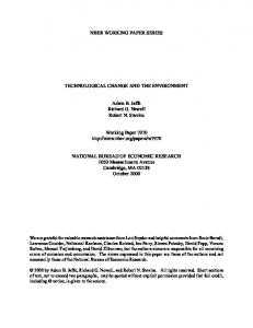
not only from the creators of the new knowledge but also from “user preferences” resulting in so-called market niches [34]. Examples of this are found in the computer industry where the DOS/Wintel PC and Macintosh computers have coexisted in the market place for a long period of time because each type of computer has a niche defined by user preferences (Apple computers have survived in the marketplace because Apple created a niche for itself by focusing on graphics, an area DOS was not concentrating on). Coexistence of technologies is probably the least explored aspect of technological dynamics. Nair et al. [28] argue from real cases in the industry, that the complexity of the underlying technology, ecological and institutional dynamics may allow coexistence regimes of competing technologies. Watanabe et al. [41] analyzes a complex interplay between competitive and cooperative species in an ecosystem based in the Lotka-Volterra equations. This dynamic resembles the co-evolution process in an ecosystem where, in order to maintain sustainable development, a complex interplay between competition and cooperation, typically observed in prey-predator systems, sets in. Although all these topics have been the subject of empirical and theoretical work, they have usually been considered in isolation with an emphasis on the process of technological substitution. In this paper we introduce a biologically motivated model that explicitly accounts for the emergence, replacement and coexistence of technological innovations. We couple the adoption of a technology with the efficiency in technology absorption and the provision of financial resources (actual or potential resources that allow an organization to adapt successfully to internal and external pressures for change in technologies or markets); this resource is limited but not constant and is utilized at a constant rate. The framework is a rich alternative for the theoretical basis of innovation diffusion where models generally assume a logistic equation (constant carrying capacity) modified to account for variable carrying capacity through the introduction of a factor known as “external” innovation. This approach is not complete since actual resources (which are dynamic entities in themselves) can also alter the carrying capacity not only through the inflow of external adopters. Besides this somewhat obvious justification, the model is capable of explaining the existence of several closely related technologies, coexisting without necessarily competing out each other. To complete our study we use an Adaptive Dynamic framework [39], [10], [24]. Adaptive dynamics has been a standard tool to give an evolutionary perspective to ecological and technology models in order to obtain a view of the role of “natural selection” in shaping the characteristics of a life cycle [7]. In this sense in a competitive system the generation of new technology produces the emergence of technological variety. 1.1. Examples of the technology adoption. Figure 1 shows the number of patents issued in the area of climate change mitigation technologies such as solar photovoltaic (solav PV), solar thermal (solar TH), wind, biofuels among others. The patent data have been extracted from the EPO/OECD (European Patent Office/Organisation for Economic Co-Operation and Development) World Patent Statistics database (OECD, 2010) and cover a selection of technology fields (renewable energy) for all countries in the years from 1978 to 2006. The phenomenon of coexistence can be appreciated in renewable energy technologies in which the solar photovoltaic patents grow faster than other patents in general.

3302


According to the OECD, in the area of low-carbon technologies “innovation activity in low-carbon technologies grew dramatically after the Kyoto Protocol agreement” and “the international community will be critical for business investment decisions in R&D for low-carbon technologies and infrastructure” [30]. This supports the idea that, at least in part but importantly, the Kyoto protocol lead to an increase of innovation in these areas. 9 8

Solar PV

7

Wind

Patenting rate

6

CO2

5

Biofuels

4

Hydro

3

Geothermal

2

Solar TH

1 0 1978

1982

1986

1990

1994

1998

2002

2006

Kyoto Protocol

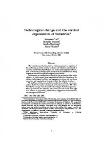
Figure 1. Innovation in Climate Change Mitigation Technologies, data were normalised to 1978=1. Based on data extracted from the EPO Worldwide Patent Statistical Database. Another example concerning the technological substitution is from monochrome to color TV systems. We show in Figure 2 that as the price of color TV sets declined, people started to switch from monochrome to color TV because the performance of color TV sets is clearly superior to monochrome TV sets. Consequently, color TV sets diffused rapidly in line with a logistic growth. They exhibited rapid growth from 1968, 8 years after their inauguration, by substituting monochrome TV sets altogether by the early 1980s. Since the technical standard for the color TV broadcasting was compatible to monochrome TV sets, people could receive color TV broadcasting through their monochrome TV sets as monochrome TV programs. In this sense, color TV broadcasting and monochrome TV broadcasting were in a competitive relationship because people could choose either monochrome or color TV sets according to their preferences. The phenomenon of substitution was expected because at a branching point the old and the new versions of the technology coexist under different resource management schemes. From these two study cases we see that our approach can provide an evolutionary interpretation about the persistence of closely related technologies (coexistence) and competitive exclusion. The paper is organized as follows. In the next section we present a model of innovation and resource supply; in particular we show a generalization of the model by allowing external influences to affect the diffusion of innovation. Then we present


3303

100

Diffusion level

80

Color TV 60

Monochrome TV

40

20

0 1966

1971

1976

1981

Figure 2. Trends in the diffusion process of TV sets in Japan. Source: Consumer Confidence Survey, Cabinet Office, Government of Japan. Adapted from Watanabe et al. (2004). the equilibrium points and stability conditions and an adaptive dynamic equation derived and analyzed with the aim of characterizing the transition between technological coexistence and extinction of a technology. Finally we present our conclusions about the purpose of this study. 2. A mathematical model for innovation and resource supply. We follow [24] adopting their approach to the context of innovation diffusion. The basic tenet of the model is that it takes time for innovations to diffuse in a given target population. Let p(t) be the proportion of adopters at time t (called the adoption curve) i.e. p(t) is a measure of the market share in terms of the approval of a product or technology. This leads to the logistic Verlhust-type growth scenario d p = rp(1 − p), (1) dt where 0 ≤ p ≤ 1, and we have rescaled the variables so as to have a carrying capacity of 1; r is the instantaneous growth rate of new adopters within the group. This model assumes that the marketplace in which the innovation can diffuse is limited by a maximum number of adopters; equation 1 is a very well known model in the innovation literature. If p(0) = p0 the above ordinary differential equation has the solution p(t) =

p0 ert →1 1 + p0 (ert − 1)

as

t→∞

(2)

illustrated in Fig. 3. If p0 < 1, p(t) simply increases monotonically to 1 while if p0 > 1 it decreases monotonically to 1 provided r > 0. In the former case there is a qualitative difference depending on whether p0 , the initial condition, satisfies either p0 > 1/2 or p0 < 1/2. For p0 < 1/2 the form has a typical sigmoid curve which is commonly observed in learning processes. The parameters p0 and r have to be

3304


estimated from historical data. The results and conclusions that can be derived from 1 are standard and we refer the reader to [42], [13] for more information. The function p(t) is a S-shaped curve (see [42]) for certain parameters values, that is able to describe the birth, growth, and depletion of a technology [29], [11]. The classical interpretation of this curve says that in the initial period there is much experimentation in the product, gradually establishing a position in the market and among early users. Thereafter there is a kind of economic takeoff to a period of incremental improvements accelerated in quality, efficiency and cost effectiveness, then the process finds its limits. At this point the technology reaches maturity, it has lost its dynamism and profitability (see Fig. 3). This state may continue for months, years or decades. Upon reaching maturity it is very likely that the product will be replaced.

1.2

0.05

0.045

Late diffusion

1

0.04 Cumulative frequency distribution (total adoptions)

0.8

0.035

0.03

0.6

0.025

0.02 0.4

0.015

Initial diffusion

0.2

Frequency distribution (new adoptions events)

0.01 0.005

0

0 0

2

4

6

8

10

12

time

Figure 3. S-Shaped curve and frequency distribution by the adopters function p(t) with p0 = 0.01 and r = 0.9. A example of S-shaped curve in real data is the use of patent citations as an indicator of knowledge flow, extensively discussed in [18], [19] and references therein. The patents are used as surrogates of the creation of new ideas, and the citations that patents make to previous patents are indicators of existing ideas used in the creation of new knowledge, i.e., adoption. These models are based on the citation functions (citation frequency as a function of time elapsed from the potentially cited patent), in which the citations display a pattern of gradual diffusion and ultimate obsolescence. The dynamics of adoption of a new technology are not isolated, as the model above implicitly assumes, but are immersed, in particular, in the economic conditions that prevail and define the magnitude of the parameter r. In general, the growth rate r depends on several factors, in particular, on the resources (prominently financial but also cultural, economical, etc.) exclusively allocated for the enhancement of the adoption of the innovation. The size of this resource budget we represent by ω which can take values, after rescaling, on 0 ≤ ω ≤ 1. The simplest hypothesis that describes the dependence of


3305

the growth rate of the adopters on the budget is a linear dependence: r(ω) = nω − m

(3)

where n is the instantaneous rate of technology adoption and m is the rate at which a technology is abandoned, where n ≥ m. Note that the dimensions of n and m are 1/time (note that ω is adimensional after rescaling) which is consistent with the units of the adoption rate. This relation says that the adoption rate increases in direct proportion to the size of the allocated present budget and decreases according to adoption failure. We now have to establish the budget dynamics [24]. Here we will be assuming that the budget has a limiting size set by the investors in advance of the market introduction of the technology and equal to λ; we also assume that investors invest by allocating resources to the budget in direct proportion to the not yet allocated budget, that is, to 1 − ω; finally, the budget is used or consumed by adopters at a rate npω where n is the efficiency with which resources are converted into technology adopters. Therefore, the term assumes that budget or resource use is proportional to the product of instantaneous rate of technology adoption n and pω that represents the interaction between adopters and resources (following a law of mass action implicit also in equation 1): d ω = λ(1 − ω) − pωn. dt

(4)

In the absence of adopters, p = 0, the resources are thus described as ω(t) = 1 − e−λt where one can see that the resources saturate to a maximum amount of 1. Following [24], the model with resource renewal corresponds to the following equations with given non-zero initial conditions for p and ω d p dt d ω dt

=

(nω − m)p(1 − p),

(5)

=

λ(1 − ω) − pωn.

(6)

We adapt an ecological perspective to explain the technology cycle model. The link between these two views is that the interplay between technological change and innovation is akin to the process of evolution by natural selection in which competition between individuals in the same population or individuals of different species is the most important mechanism. For that reason as in the ecological context, the limited amount of resources is the root of competition, which in technology innovation becomes the level of financial resources available to adopt a technology. The model admits three different asymptotic outcomes. The calculation of equilibrium points is straightforward. We limit ourselves to a reinterpretation of the equilibria originally obtained in [24] to the case of the innovation process discussed here. a. Adoption failure. The equilibrium E = (0, 1) is stable. Here, the adopters vanish pˆ0 = 0, but since there is a constant supply budget, it goes to its allowable maximum ω ˆ 0 = 1, unused. This is an scenario where technology adoption fails but not for lack of resources. This equilibrium is stable when the adoption rate is inefficient (perhaps the technology is difficult to assimilate [37], [14]) meaning that m > n making r < 0 possibly indicating that a maladaptive or bad strategy was implemented making it possible to reach the value ω ˆ 0 = 1.

3306


b. Incomplete adoption. In this case the adopters in the long term go to an λ(1− m n ) equilibrium given by pˆ1/2 = , while the resource level has an equilibrium m m 1/2 equal to ω ˆ = n . Here adopters do not saturate the market and do not exhaust the budget allocated to adoption (see Fig. 4); the abandonment rate of technology is lower than the instantaneous rate of adoption, m < n, thus generating a net increase through time. In this scenario the adopters will stabilize at a level that is not the maximum allowable (i.e., there will be people left to adopt); likewise the budget stabilizes at a certain level that is not the maximum. λ < m This equilibrium is stable for investment strategies satisfying λ+n n < 1 which could be achieved if the efficiency of transforming resources into adopters is high (n large). Another way of describing the above is through the inequality: 1 1 >λ − . m n This indicates that in order for (b p1/2 , ω b 1/2 ) to be stable, the efficiency rate must be greater than the supply of resources λ during the time where adoption is actively 1 taking place m − n1 .

Figure 4. Incomplete adoption. Top: Evolution for technology dynamic with resources renewal with initial conditions p0 = 0.01, ω0 = 0.01. Continuous line and dash line represent the time evolution of the budget and adopters respectively. Bottom: Phase plane of (b p1/2 , ω b 1/2 ). The parameters are n = 0.6, m = 0.35, λ = 0.34, = 0.9, pb1/2 = 0.4497 and ω b 1/2 = 0.5833. c. Full adoption. We can observe that in Fig. 5 the adopters stabilize at the λ maximum, pˆ1 = 1 while the budget or economic resources settle to ω ˆ 1 = λ+n . Notice that this scenario indicates that the technology was successful because it saturates the marketplace although there is still a bit of resources untouched. Note that if efficiency is low (n small) then the leftover budget will be small; in fact only


3307

λ if efficiency is low is this equilibrium reachable since 0 ≤ m n ≤ λ+n is required in this case. It is important to point out that incomplete adoption and full adoption interchange stability: when one is stable the other is unstable and vice versa. Incomplete adoption sets the stage for the possibility of coexisting technologies without the dominance of one, in other words there are resources for the standard life cycle of creative destruction to take place.

Figure 5. Full adoption. Top: Evolution for technology dynamic with resources renewal and initial conditions p0 = 0.01, ω0 = 0.01. Continuous line and dash line represent the time evolution of the budget and adopters respectively. Bottom: Phase plane of (b p1 , ω b 1 ), 1 the parameters are n = 0.85, m = 0.23, λ = 0.25, = 0.5, pb = 1 and ω b 1 = 0.3703

In summary, the important observation is that the very act of adopting the technology leaves resources that could be used to adopt another competing technology that could, in principle, displace the one that made possible its existence; moreover if the use of resources is efficient, more resources will be left available for other technologies. Also depending on the efficacy of resource use either we have a stable full adoption or a stable incomplete adoption. In the following table we show the conditions that need to be satisfied for each of the scenarios to be stable. We are interested is the analysis of the transition between full technology adoption (case c) and incomplete adoption (case b) since the latter can induce technological diversification as will be described shortly. Note that feasible and interesting cases occur only when 0 ≤ m n ≤ 1, i.e. the , this represents the adopters important parameter for stability of the system is m n that leave the technology during the time that it takes to adopt with m < n.

3308


Strategy m>n m λ λ+n < n < 1 m λ 0 ≤ n ≤ λ+n

Equilibrium States Adoption failure (ˆ p0 , ω ˆ 0) 1/2 Incomplete adoption (ˆ p ,ω ˆ 1/2 ) 1 Full adoption (ˆ p ,ω ˆ 1)

Table 1. Equilibrium states for the dynamics of technology adopters in a system with economic resource renewal. 2.1. Innovation with external sources. Before we continue with the analysis of our model, in this section we take a quick look at the classical introduction of “external” adoption. A traditional approach for describing this system is based on the Bass model [2], where there is an important distinction in adopters: innovators versus imitators. Innovators are not influenced in the timing of their initial purchases by the number of people who have already bought the product, while imitators are influenced by the number of previous buyers [2], [42]. In this case the biological analogy breaks down and the innovation scenario leads to a different interpretation [6], [23]. The basic model parameters are the same: let r be the instantaneous rate at which a current non-adopter hears about (and adopts) the innovation from a previous adopter within the group, and let r∗ be the instantaneous rate at which the potential adopter hears about (and adopts) it from sources outside of the group; r and r∗ are nonnegative and not both zero, so the model is set up in terms of innovation and imitation behavior. The adopters dynamic is modeled now as d p = (rp + r∗ )(1 − p). dt

(7)

When r and r∗ are constant the solution to the above is p(t) =

1 − e−(r+r∗ )t . 1 + rr∗ e−(r+r∗ )t

The above function is also a S-shaped curve (for certain parameters values), the total growth rate r + r∗ , and in the absence of adopters inside the system (r = 0) adoption can still take place provided the initial condition is positive. Here the function p(t) is a measure of the market share over time from internal and external sources. Define r∗ (ω) = n∗ ω − m∗ and r(ω) = nω − m, as before, to represent the adopters increase rate as a function of external and internal processes where both depend on the same source of financing. As before n and n∗ are the instantaneous rates of adoption, m and m∗ are the abandonment rates of technology. We then have the following system d p dt d ω dt

=

(rp + r∗ )(1 − p),

= λ(1 − ω) − pω(n + n∗ ).

(8) (9)

The equilibrium points are now a bit more complicated to express than before since the effect of external influences imposes feasibility boundaries (functions of the parameters) on the variables that determine the validity and technological significance of the model predictions. We deal with this in detail in the Appendix. For now a


3309

quick analysis gives one of the equilibrium points: λ pˆ1 = 1, ω ˆ1 = (10) λ + (n + n∗ ), that corresponds to the case of successful innovation although with restrictions not present in our model (5)-(6). After some straightforward but nevertheless cumbersome algebraic manipulations (see Appendix) one finds the additional equilibrium point: r∗ (ω1 ) , ω ˆ 1/2 = ω1 . (11) pˆ1/2 = − r(ω1 ) where ω1 is shown in the Appendix. The interpretation of these equilibrium scenarios is the same as the one given in section 2 except for the case of incomplete adoption since here, we have a further restriction: either r∗ or r is negative, that is, the instantaneous growth rate per adopter from external or internal sources is negative. Moreover a stability condition for the equilibrium point (11) is |r∗ (ω)| ≤ |r(ω)|, which means that in absolute value, the instantaneous growth rate at which an adopter knows about an innovation outside of the group must be less than instantaneous growth rate within the group. This means that only if technological adoption is very inefficient inside or outside the group, is incomplete adoption feasible. Therefore in what follows we only discuss the full adoption stability properties. Full Adoption. At this point we have the maximum of adopters (see Fig. 6) because this scenario indicates that the technology was successful. This equilibrium is stable when 1 1