The Efficiency of a Homology Algorithm based on Discrete Morse Theory and Coreductions (Extended Abstract) Shaun Harker1 , Konstantin Mischaikow1 , Marian Mrozek2 Vidit Nanda1 , Hubert Wagner2 , Mateusz Juda2 and Pawe!l D!lotko2 1
Rutgers University, Department of Mathematics, Piscataway, New Jersey, USA 2 Uniwersytet Jagiellonski, Instytut Informatyki, Krak´ ow, Poland.
[email protected],
[email protected],
[email protected],
[email protected],
[email protected],
[email protected],
[email protected]
Abstract Two implementations of a homology algorithm based on the Forman’s discrete Morse theory combined with the coreduction method are presented. Their efficiency is compared with other implementations of homology algorithms. Keywords: efficient homology algorithms, Discrete Morse theory, coreductions
1
Introduction
Homology theory is already more than 100 years old but, despite its origins in the theory of differential equations, until late 20th century it was considered a purely theoretical part of mathematics. However, in recent years homological methods found their way into the applied sciences. This causes growing demand for efficient homology algorithms. In principle, homology is an algebraic method and Smith diagonalization of integer matrices is the classical tool for computing homology. Unfortunately, because the size of inputs in many practical problems is hundred thousands and more, Smith diagonalization, which is supercubical, is to slow for many applications. Among such applications are in particular many problems in material science [6, 13, 21, 26] and imaging [5, 12, 24, 25, 28, 27]. Based on these limitations of the Smith normal form algorithm, it is not surprising that more efficient algorithms for the computation of homology have been developed over the years, see for example [7, 8, 9, 11, 16, 17, 15, 19, 20, 22], as well as the references therein. Among the many ways to overcome this problem the fundamental one is to try to improve the efficiency of Smith diagonalization [8]. However, when computing homology of spaces there is an alternative based on the so called reduction methods. The idea is to transform the original input into one which is considerably smaller and still has the same homology, and then to apply the Smith normal form algorithm as a last step. A variety of different reduction methods have been proposed such as elementary reductions, acyclic subspace reductions [20], as well as coreductions [19]. Implementations of these algorithms are available from [1, 2]. Several researchers agree that the discrete Morse theory for finite, regular CW complexes, developed by R. Forman [10], may potentially be used as a powerful reduction method (see in particular [23]). However, since the ideas are not algebraic but geometric, their implementation is not straightforward. Maybe this is the reason that although the discrete Morse theory is already 12 years old, we know of no implementation, and particularly no competitive implementation, of a homology algorithm based on the discrete Morse theory. The aim of this paper is to show that in practice applying the discrete Morse theory to computing homology of spaces indeed leads to very efficient algorithms. We present two recently
41
coded implementations of such homology algorithms in which the construction of the discrete Morse function utilizes the concept of coreductions introduced in [19]. Here we briefly describe the algorithm and show the efficiency of the two implementations. Theoretical foundations of the presented method, including a computational approach to maps induced in homology based on discrete Morse theory will be presented in [14].
2
Discrete Morse Theory
We begin with briefly recalling the fundamentals of the discrete Morse theory as developed by R. Forman [10]. Let K be the collection of cells of a finite, regular, CW complex which we will also denote by K. We denote by dim σ the dimension of the cell σ ∈ K and we write Kn for the subcollection of cells of dimension n. The adherence relation is defined by τ ≺ σ ⇔ τ ⊂ σ and dim τ = dim σ − 1 and the adherence digraph by (K, { (σ, τ ) | τ ≺ σ }). We also write bdK σ
cbdK σ
:= :=
{ τ | τ ≺ σ },
{ ρ | σ ≺ ρ }.
Forman [10] defines f : K → Z to be a discrete Morse function if for every σ ∈ K c+ (σ) := card { ρ ∈ cbd σ | f (ρ) ≤ f (σ) } ≤ 1 and
c− (σ) := card { τ ∈ bd σ | f (τ ) ≥ f (σ) } ≤ 1.
A cell σ ∈ K is critical if c+ (σ) = c− (σ) = 0. A discrete vector field V on K is a collection of pairs (τ, σ) ∈ K2 such that τ ≺ σ and each element of K is in at most one pair in V . The V -digraph of K is the adherence graph of K with the direction reversed on the elements of V . Theorem 2.1 (Forman, 1998) If f : K → Z is a discrete Morse function then { (τ, σ) ∈ K2 | τ ≺ σ and f (τ ) ≥ f (σ) } is a discrete vector field on K, called the gradient vector field of f . Theorem 2.2 (Forman, 1998) A discrete vector field V is the gradient vector field of a discrete Morse function if and only if the V -digraph of K is acyclic, ie. contains no non-trivial directed loops. We now assume that a discrete Morse function f on K is given and V is the associated gradient vector field. We introduce the following sets Q(K) := Q(K, V )
:=
K(K) := K(K, V )
:=
A(K) := A(K, V )
:=
{ τ ∈ K | ∃σ ∈ K (τ, σ) ∈ V },
{ σ ∈ K | ∃τ ∈ K (τ, σ) ∈ V }, K \ Q(K, V ) \ K(K, V ).
Note that A(K) consists precisely of critical elements of K. The fact that V is a gradient vector field causes that the elements of Q(K) and K(K) appear in pairs, which allows us to define the pairing: Q(K) ∪ K(K) + σ → σ ∗ ∈ Q(K) ∪ K(K)
42
such that if σ ∈ Q(K) then σ ∗ ∈ K(K) and if σ ∈ K(K) then σ ∗ ∈ Q(K). Let C(K) be the chain complex of K (see [18, Chapter IX.5]) and let ,·, ·- denote the scalar product associated with the free basis K. If τ ≺ σ, then τ has a non-zero coefficient in the boundary chain of σ, called the incidence number of the pair (σ, τ ). We denote it by κ(σ, τ ). The weight of a pair (σ, τ ) ∈ K2 is defined by τ ≺σ κ(σ, τ ) w(σ, τ ) := −κ(τ, σ)−1 τ . σ 0 otherwise.
A path from σ ∈ K to τ ∈ K is a sequence α = (α0 , α1 , . . . , αn ) ∈ Kn+1 such that (αi−1 , αi ) ∈ V , α0 = σ and αn = τ . The path α is alternating if dim αi = dim α0 − (i
mod 2).
We denote the set of all paths from σ ∈ K to τ ∈ K by PV (σ, τ ) and the set of alternating paths from σ ∈ K to τ ∈ K by PVa (σ, τ ). The weight of a path α = (α0 , αa , . . . , αn ) is given by w(α) :=
n %
w(αi−1 , αi ).
i=1
& ' We define the Morse complex (M, ∆) := Mq (K, V ), ∆q (K, V )q∈Z of a gradient vector field V on K by Mq
:=
,∆q σ, τ -
:=
{ σ ∈ A(K) | dim σ = q } ( w(α).
(1) (2)
α∈PVa (σ,τ )
The central theorem of the discrete Morse theory is the following theorem. Theorem 2.3 (Forman, 1998)
H∗ (K) ∼ = H∗ (M, ∆).
Now, in many applied situations one expects the Morse complex (M, ∆) to be much smaller than the original complex K. Therefore, computing the homology of the Morse complex instead of the original complex may substantially reduce the amount of necessary algebraic computations and consequently lead to a particularly efficient homology algorithm. However, for this to work one needs an efficient method of constructing a discrete Morse function.
3
Discrete Morse Function Construction based on coreductions as a tool for computing homology.
The coreduction homology algorithm, in the sequel referred to as CR homology algorithm, presented in [19] is among the most efficient homology algorithms for cubical sets available so far. Recall that a pair (σ, τ ) ∈ K2 is called a coreduction pair if bdK s = {t}. It is proved in [19] that in the context of so called S-complexes (see [19, Section 2]) a coreduction pair may be removed from K without changing the homology of K. Roughly speaking, the CR homology algorithm consists in removing coreducton pairs as long as they are available. However, one easily sees that in a compact CW complex no coreduction pairs exists. Nevertheless, if K is a CW complex and v is a vertex of K then K \ {v} is an S-complex which admits coreduction pairs. Since we have ¯ H(K \ {v}) ∼ = H(K, {v}) ∼ = H(K)
43
(3)
Algorithm 3.1 discreteMorseFunction(CW complex K) V := L := A := K := Q := dom f := ∅; while K 1= ∅ do if L = ∅ then n := min { q | Kq 1= ∅ }; move an element r from Kn to A; define f (r) as 1 + max { f (r$ ) | r$ ∈ dom f, r$ ≺ r }; enqueue(L, cbdK r); else s:=dequeue(L); if bdK s = {t} then move s from K to K and t from K to Q; insert (s, t) to V ; define f (s) and f (t) as 1 + max { f (s$ ) | s$ ∈ dom f, s$ ≺ s }; enqueue(L, cbdK t); else if bdK s = ∅ then enqueue(L, cbdK s); endif ; endif ; endwhile ;
Table 1: Discrete Morse Function by coreduction method ¯ with H(K) standing for the reduced homology of K and ) ¯ 0 (K) if n = 0, Z⊕H Hn (K) = ¯ n (K) H otherwise,
(4)
it is sufficient to compute H(K \ {v}) instead of H(K). We refer the reader to [19] for details. The efficiency of the CR homology algorithm crucially depends on the amount of cells left after all available coreduction pairs are removed. One can show that if after removing a vertex from a connected CW-complex K all available coreduction pairs have been removed then the remaining complex has no vertices. Then, often removing an edge causes that the coreduction pairs reappear. However, in this case there is no simple relation between the homology before and after removing an edge as in the case of formulas (3) and (4). But the coreduction technique may be used to construct a discrete Morse function on K. The respective algorithm is presented in Table 1. Theorem 3.2 Algorithm 3.1 runs in linear time. The coreduction based, discrete Morse theory homology algorithm, referred in the sequel as DMT algorithm, consists in applying Algorithm 3.1 to a a finite, regular, CW complex K followed by the construction of the respective Morse complex and computation of its homology by algebraic methods. Note that a straightforward, naive implementation of formula (2) may lead to heavy computations and consequently the gains from the approach may not show up. An algorithm for the boundary operator ∆ used in our implementations is considerably more efficient than Forman’s sum over paths formula. It will be presented elsewhere.
4
Numerical experiments
We have two independent implementations of CR algorithm and DMT algorithm. The first is by S. Harker and will be available soon from CHOMP [2]. The other is by H. Wagner, M. Juda, P.
44
dim size in millions H0 H1 H2 H3 H4 Linbox::Smith RedHom::Shave+Linbox::Smith ChomP RedHom::CR ChomP::DMT ChomP::CR+DMT RedHom::CR+DMT
T × S1 5 0.07 Z Z3 Z3 Z
(S 1 )3 6 0.10 Z 0 0 Z
S1 × K 6 0.40 Z Z2 + Z2 Z + Z2
130 0.5 1.3 0.03 0.06 0.04 0.02
350 0.1 1.7 0.04 0.15 0.16 0.08
> 600 2.2 10 0.26 1.6 1.7 0.5
T ×T 6 2.36 Z Z4 Z6 Z4 Z > 600 > 600 56 2.5 5.9 3 1.1
Table 2: The homology and the timings in seconds for a collection of cubical manifolds. The consecutive rows contain: the manifolds, the embedding dimension, the number of cells counted in millions, the homology groups and the timings for various implementations of homology algorithms.
dim size in millions H0 H1 H2 Linbox::Smith RedHom::Shave+Linbox::Smith ChomP RedHom::CR ChomP::DMT ChomP::CR+DMT RedHom::CR+DMT
P0001 3 75.56 Z7 6554 Z Z2 > 600 > 600 400 36 110 45 26
P0050 3 73.36 Z2 2962 Z
P0100 3 71.64 Z Z1057
> 600 > 600 360 34 110 43 25
> 600 > 600 310 33 100 42 24
Table 3: The homology and the timings in seconds for a collection of cubical sets arising from the numerical simulation of Cahn-Hillard partial differential equation. The consecutive rows contain: the names of sets, the embedding dimension, the number of cells counted in millions, the homology groups and the timings for various implementations of homology algorithms. D$lotko and M. Mrozek and will be available soon as RedHom sublibrary [3] of CAPD [1]. Both implementations are written in C++. We have compared the performance of these implementations, as well as the combination of CR followed by DMT, with our earlier best algorithms and with the classical approach utilizing Smith diagonalization available form LinBox [4]. We chose four collections of sets for our tests: a collection of five and six dimensional cubical manifolds, a collection of huge cubical sets arising from numerical simulations of Cahn-Hillard partial differential equation and a collection of random cubical sets in dimension four. For comparison purposes we chose the following implementations of homology algorithms Linbox::Smith - the classical homology algorithm based on the LinBox [4] implementation of Smith diagonalization
45
dim size in millions H0 H1 H2 H3 Linbox::Smith RedHom::Shave+Linbox::Smith ChomP RedHom::CR ChomP::DMT ChomP::CR+DMT RedHom::CR+DMT
d4s8f50 4 0.07 Z2 Z2 174 Z Z2 120 4 1 0.08 0.05 0.03 0.03
d4s12f50 4 0.34 Z2 Z17 1389 Z Z15 > 600 > 600 8.3 1.4 0.38 0.16 0.16
d4s16f50 4 1.04 Z2 Z30 5510 Z Z71 > 600 > 600 41 15 1.8 0.56 0.58
d4s20f50 4 2.48 Z2 Z51 15401 Z Z179 > 600 > 600 170 140 5.3 1.4 2.9
Table 4: The homology and the timings in seconds for a collection of random cubical sets. The consecutive rows contain: the names of sets, the embedding dimension, the number of cells counted in millions, the homology groups and the timings for various implementations of homology algorithms. RedHom::Shave+Linbox::Smith - as Linbox::Smith but preprocessed by the method of shaving in the spirit of [20, Section 7] in order to speed up the computations ChomP - the main homology engine available from CHOMP [2] based on the implementation by P. Pilarczyk RedHom::CR - the implementation by M. Mrozek of the CR homology algorithm [19] for RedHom sublibrary of CAPD [1] and CHOMP [2]. ChomP::DMT - the implementation by. S. Harker of DMT homology algorithm for CHOMP [2]. ChomP::CR+DMT - a combination of the CR homology algorithm followed by DMT homology algorithm implemented by S. Harker for CHOMP [2]. RedHom::CR+DMT - a combination of the CR homology algorithm followed by DMT homology algorithm implemented by H. Wagner, M. Juda, P. D$lotko and M. Mrozek for RedHom sublibrary [3] of CAPD [1]. The homology of the examples and the timings for the selected implementations are presented in Tables 2, 3 and 4. The tests were performed on a 3.0GHz Intel Xeon processor with 16GB of RAM running Linux. Note that in the case of Linbox based implementations we present only the timing of the Smith diagonalization of the matrices of boundary maps. In this case the actual time needed to compute the homology is longer, since the time needed to generate the matrices of boundary maps and (in the case of RedHom::Shave+Linbox::Smith) the preprocessing time should be added. Tables 2, 3 and 4 indicate that DMT homology algorithm may be a valuable alternative to the existing methods, although a combination of CR homology algorithm followed by DMT homology algorithm may be even better. Most likely this is because DMT homology algorithm, unlike CR homology algorithm, requires storing all the coreduction pairs processed, because they are needed in the construction of the Morse complex. On the other hand, in the case of CR homology algorithm each spotted coreduction pair may be immediately removed. The implementations are primarily aimed at cubical sets but they are written using generic methods so we tested them also on a collection of three simplicial complexes. The results are
46
dim size in millions H0 H1 H2 H3 H4 ChomP RedHom::CR+DMT
random set 4 4.8 Z Z39 Z84
Bj¨orner set 2 1.9 Z 0 Z
830 65
310 11
S5 5 4.3 Z 0 0 0 Z 2100 100
Table 5: The homology and the timings in seconds for a collection of simplicial complexes. The consecutive rows contain: the names of sets, the embedding dimension, the number of cells counted in millions, the homology groups and the timings for various implementations of homology algorithms. available in Table 5. We also tested these examples with the classical Smith diagonalization method based on [4] but in each case we failed to get results either due to lack of memory of very long waiting times. However, these results are very preliminary and DMT homology algorithm must be tested on a larger collection of simplicial complexes to draw some conclusions. Summing up, allthough we cannot claim that discrete Morse theory provides a universal solution for fast homology computations, we believe that DMT homology algorithm, and particularly the combination of CR and DMT homology algorithms may be very helpful in computing homology of many huge sets appearing in concrete problems. Acknowledgments. SH, KM and VN are partially supported by AFOSR, DARPA, NSFDMS0915019 and NSF-CBI 0835621. MM and MJ are partially supported by MNiSW grant N N201 419639. HW is partially supported by MNiSW grant N N201 419639 and by the Austrian Science Fund (FWF) grant no. P20134-N13. PD is partially supported by MNiSW grant N N206 625439.
References [1] CAPD: Computer assisted proofs in dynamics, http://capd.ii.uj.edu.pl/. [2] CHOMP: Computational homology project, http://chomp.rutgers.edu/. [3] CAPD::RedHom: Reduction homology algorithms, http://redhom.ii.uj.edu.pl/. [4] Project linbox: Exact computational linear algebra, http://www.linalg.org/. [5] M. Allili, K. Mischaikow, and A. Tannenbaum. Cubical homology and the topological classification of 2d and 3d imagery. IEEE International Conference on Image Processing, 2:173–176, 2001. [6] Dirk Bl¨omker, Stanislaus Maier-Paape, and Thomas Wanner. Phase separation in stochastic Cahn-Hilliard models. In Alain Miranville, editor, Mathematical Methods and Models in Phase Transitions, pages 1–41. Nova Science Publishers, New York, 2005. [7] Cecil Jose A. Delfinado and Herbert Edelsbrunner. An incremental algorithm for betti numbers of simplicial complexes. In SCG ’93: Proceedings of the ninth annual symposium on Computational geometry, pages 232–239, New York, NY, USA, 1993. ACM. [8] Jean-Guillaume Dumas, Frank Heckenbach, David Saunders, and Volkmar Welker. Computing simplicial homology based on efficient Smith normal form algorithms. In Algebra, geometry, and software systems, pages 177–206. Springer, Berlin, 2003.
47
[9] Herbert Edelsbrunner, David Letscher, and Afra Zomorodian. Topological persistence and simplification. Discrete & Computational Geometry, 28(4):511–533, 2002. [10] Robin Forman. Morse theory for cell complexes. Advances in Mathematics, 134:90–145, 1998. [11] J. Friedman. Computing Betti numbers via combinatorial Laplacians. 21(4):331–346, 1998.
Algorithmica,
[12] P. Frosini and C. Landi. Size theory as a topological tool for computer vision. Pattern Recognition And Image Analysis, 9(4):596–603, 1999. [13] Marcio Gameiro, Konstantin Mischaikow, and Thomas Wanner. Evolution of pattern complexity in the Cahn-Hilliard theory of phase separation. Acta Materialia, 53(3):693–704, 2005. [14] Shaun Harker, Konstantin Mischaikow, Marian Mrozek, and Vidit Nanda. Computing homology via Morse coreductions. in preparation. ´ [15] T. Kaczy´ nski, M. Mrozek, and M. Slusarek. Homology computation by reduction of chain complexes. Computers & Mathematics with Applications, 35(4):59–70, 1998. [16] Tomasz Kaczynski, Konstantin Mischaikow, and Marian Mrozek. Computing homology. Homology, Homotopy and Applications, 5(2):233–256, 2003. [17] Tomasz Kaczynski, Konstantin Mischaikow, and Marian Mrozek. Computational Homology, volume 157 of Applied Mathematical Sciences. Springer-Verlag, New York, 2004. [18] W.S. Massey. A Basic Course in Algebraic Topology Applied Mathematical Sciences, 157. Springer-Verlag, New York – Berlin – Heidelberg, 1991. [19] Marian Mrozek and Bogdan Batko. Coreduction homology algorithm. Discrete & Computational Geometry, 41(1):96–118, 2009. ˙ [20] Marian Mrozek, Pawe$l Pilarczyk, and Natalia Zelazna. Homology algorithm based on acyclic subspace. Computers & Mathematics with Applications, 55(11):2395–2412, 2008. [21] Marian Mrozek and Thomas Wanner. Coreduction homology algorithm for inclusions and persistent homology. Computers and Mathematics with Applications, accepted. [22] Samuel Peltier, Adrian Ion, Yll Haxhimusa, Walter Kropatsch, and Guillaume Damiand. Computing homology group generators of images using irregular graph pyramids. Lecture Notes in Computer Science, 4538(3):283–294, 2007. [23] Francis Sergeraert. W-reductions. personal communication. [24] A. Szymczak, A. Stillman, A. Tannenbaum, and K. Mischaikow. Coronary vessel trees from 3d imagery: A topological approach. Med Image Anal., 10(4):548–559, 2006. [25] A. Verri and C. Uras. Metric-topological approach to shape representation and recognition. Image Vision Comput., 14:189–207, 1996. [26] Thomas Wanner, Edwin R. Fuller Jr., and David M. Saylor. Homological characterization of microstructure response fields in polycrystals. Acta Materialia, 58(1):102–110, 2010. ˙ [27] M. Zelawski. Pattern recognition based on homology theory. Machine Graphics & Vision, 14(3):309–324, 2005. [28] D. Ziou and M. Allili. Generating cubical complexes from image data and computation of the euler number. Pattern Recognition, 35(12):2833–2839, 2002.
48