http://www.sdsc.edu/~downey. Dror G. Feitelson ..... was submitted from June 6 to December 2, 1995 .... and Downey used a similar technique to summarize.
The Elusive Goal of Workload Characterization Allen B. Downey
Computer Science Department Colby College, Waterville, ME 04901 http://www.sdsc.edu/~downey
Abstract
The study and design of computer systems requires good models of the workload to which these systems are subjected. Until recently, the data necessary to build these models|observations from production installations|were not available, especially for parallel computers. Instead, most models were based on assumptions and mathematical attributes that facilitate analysis. Recently a number of supercomputer sites have made accounting data available that make it possible to build realistic workload models. It is not clear, however, how to generalize from speci c observations to an abstract model of the workload. This paper presents observations of workloads from several parallel supercomputers and discusses modeling issues that have caused problems for researchers in this area.
1 Introduction We like to think of building computer systems as a systematic process of engineering|we de ne requirements, draw designs, analyze their properties, evaluate options, and nally construct a working system. But in many cases the resulting products are su�ciently complex that it makes sense to study them as opaque artifacts, using scienti c methodology of observation and measurement. In particular, such observations are necessary to validate (or refute) the assumptions used in the analysis and evaluation. Thus observations made using one generation of systems can be used as a basis for the design and evaluation of the next generation. A memorable example of such a cycle occurred recently in the eld of data communications. Such communications had traditionally been analyzed using Poisson-related models of tra�c, which indicated that the variance should smooth out over time and when multiple data sources are combined. But in 1994 Leland and co-workers showed, based on extensive observations and measurements, that this does not happen in practice [27]. Instead, they proposed a fractal tra�c model that captures the burstiness of network tra�c and leads to more realistic evaluations of required bu�er space and other parameters. Analyzing network tra�c was easy, in some sense, because all packets are of equal size and the only characteristic that required measurement and modeling was the arrival process. But if we consider
Dror G. Feitelson
Institute of Computer Science The Hebrew University, 91904 Jerusalem, Israel http://www.cs.huji.ac.il/~feit
a complete computer system, the problem becomes more complex. For example, a computer program may require a certain amount of memory, CPU time, and I/O, and these resource requirements may be interleaved in various ways during its execution. In addition there are several levels at which we might model the system: we can study the functional units used by a stream of instructions, the subsystems used by a job during its execution, or the requirements of jobs submitted to the system over time. Each of these scales is relevant for the design and evaluation of di�erent parts of the system: the CPU, the hardware con guration, or the operating system. In this paper we focus on characterization of the workload on a parallel system, from an operating system perspective (as was done in [12, 38]). Thus we investigate means to characterize the stream of parallel jobs submitted to the system, their resource requirements, and their behavior. We show that such characterization must contend with various problems; some can be addressed easily, but others seem to be hard to avoid.
1.1 De nitions We use size to refer to the number of processors used by a parallel program (as shorthand for \cluster size", \partition size", or \degree of parallelism"). We use duration to refer to the span of time starting when a job commences execution and ending when it terminates (otherwise known as \runtime" or \lifetime"; it is also the same as \response time" if the job did not have to wait). The product of these two sizes, which represents the total resources (in CPU-seconds) used by the job, is called its area.
2 Modeling There are two common ways to use a measured workload to analyze or evaluate a system design: (1) use the traced workload directly to drive a simulation, or (2) create a model from the trace and use the model for either analysis or simulation. For ex-
ample, trace-driven simulations based on large address traces are often used to evaluate cache designs [23, 22]. But models of how applications traverse their address space have also been proposed, and provide interesting insights into program behavior [36, 37]. The advantage of using a trace directly is that it is the most \real" test of the system; the workload re ects a real workload precisely, with all its complexities, even if they are not known to the person performing the analysis. The drawback is that the trace re ects a speci c workload, and there is always the question of whether the results generalize to other systems. In particular, there are cases where the workload depends on the system con guration, and therefore a given workload is not necessarily representative of workloads on systems with other con gurations. Obviously, this makes the comparison of di�erent con gurations problematic. In addition, traces are often misleading if we have incomplete information about the circumstances when they were collected. For example, workload traces often contain intervals when the machine was down or part of it was dedicated to a speci c project, but this information may not be available. Workload models have a number of advantages over traces. � The modeler has full knowledge of workload characteristics. For example, it is easy to know which workload parameters are correlated with each other because this information is part of the model. � It is possible to change model parameters one at a time, in order to investigate the in uence of each one, while keeping other parameters constant. This allows for direct measurement of system sensitivity to the di�erent parameters. It is also possible to select model parameters that are expected to match the speci c workload at a given site. In general it is not possible to manipulate traces in this way, and even when it is possible, it can be problematic. For example, it is common practice to increase the modeled load on a system by reducing the average interarrival time. But this practice has the undesirable consequence of shrinking the daily load cycle as well. With a workload model, we can control the load independent of the daily cycle.
� A model is not a�ected by policies and constraints
that are particular to the site where a trace was recorded. For example, if a site con gures its NQS queues with a maximum allowed duration of 4 hours, it forces users to break long jobs into multiple short jobs. Thus, the observed distribution of durations will be di�erent from the \natural" distribution users would have generated under a di�erent policy. � Logs may be polluted by bogus data. For example, a trace may include records of jobs that were killed because they exceeded their resource bounds. Such jobs impose a transient load on the system, and in uence the arrival process. However, they may be replicated a number of times before completing successfully, and only the successful run represents \real" work. In a model, such jobs can be avoided (but they can also be modeled explicitly if so desired). � Finally, modeling increases our understanding, and can lead to new designs based on this understanding. For example, identifying the repetitive nature of job submittal can be used for learning about job requirements from history. One can design a resource management policy that is parameterized by a workload model, and use measured values for the local workload to tune the policy. The main problem with models, as with traces, is that of representativeness. That is, to what degree does the model represent the workload that the system will encounter in practice? Once we decide to construct a model, the chief concern is what degree of detail to include. As noted above, each job is composed of procedures that are built of instructions, and these interact with the computer at di�erent levels. One option is to model these levels explicitly, creating a hierarchy of interlocked models for the di�erent levels [5, 2]. This has the obvious advantage of conveying a full and detailed picture of the structure of the workload. In fact, it is possible to create a whole spectrum of models spanning the range from condensed rudimentary models to direct use of a detailed trace. For example, the sizes of a sequence of jobs need not be modeled independently. Rather, they can be derived from a lower-level model of the jobs' structures [14]. Hence the combined model will be useful both for evaluating systems in which jobs are executed on prede ned partitions, and for evaluating systems in which the partition size is de ned at
runtime to re ect the current load and the speci c � The median, which represents the center of the requirements of jobs. sequence: it is the 50th percentile, which means The drawback of this approach is that as more that half of the observations are smaller and detailed levels are added, the complexity of the half are larger. model increases. This is detrimental for two rea- � Quartiles (the 25, 50, and 75 percentiles) and sons. First, more detailed traces are needed in order deciles (percentiles that are multiples of 10). to create the lower levels of the model. Second, it These give an indication of the shape of the is commonly the case that there is wider diversity distribution. at lower levels. For example, there may be many � The semi-interquartile range (SIQR), which jobs that use 32 nodes, but at a ner detail, some of gives an indication of the spread around the them are coded as data parallel with serial and parmedian. It is de ned as the average of the disallel phases, whereas others are written with MPI tances from the median to the 25 percentile and in an SPMD style. Creating a representative model to the 75 percentile. that captures this diversity is hard, and possibly arbitrary decisions regarding the relative weight of the Mode-based. The mode of a sequence of observations is the most common value observed. This various options have to be made. statistic is obviously necessary when the values In this paper we concentrate on single-level are not numerical, for example when they are models, which may be viewed as the top level in user names. It is also useful for distributions a hierarchical set of models [14]. Even with this rethat have strong discrete components, as may striction, di�culties abound. indeed happen in practice (e.g. see Figs. 2 and 3 Statistics 4 below). The whole point of a model is to create a concise The use of moments (mean, variance, etc.) as representation of the observed workload. Thus it summary statistics is common because they are easy is desirable to derive a small set of numbers or a simple function that characterizes each aspect of the to calculate and most people have some intuition workload. If we cannot do this, we are left with the about their meaning (although this intuition starts to wane somewhere between skew, the third mooriginal data as the best representation. Any time we reduce a set of observations to a ment, and kurtosis, the fourth). small set of numbers, the result is called a summary Unfortunately, many researchers are in the statistic. These fall into three families (See Jain's habit of reporting these statistics for non-symmetric treatise for more details [19, chap. 12]): distributions. At best, this practice is misleading, Moment-based: The kth moment of a sequence since the reader's intuition about the distributions x1P ; x2; : : :xn of observations is de ned by mk = will be wrong. At worst, calculated moments are meaningless values. 1 k n xi . Important statistics derived from moThere are two reasons moments may fail to ments include � The mean, which represents the \center of grav- summarize a distribution: P ity" of a set of observations: x� = n1 xi . � Nonconvergence: For some distributions, the mo� The standard deviation, which gives an indi- ments of a sample do not converge on the mocation regarding the degree to which the ob- ments of the population, regardless of sample size. servations are spread out around the mean: An example that is common in computer science q P s = n?1 1 (xi ? x�)2 . is the Pareto distribution1 [21]. For Pareto distri� The coe�cient of variation, which is a normal- butions with shape parameter a less than 1, the mean and other moments are in nite. Of course, ized version of standard deviation: cv = s=�x. Percentile-based: Percentiles are the values that any nite sample will have nite moments, so conappear in certain positions in the sorted se- vergence is not possible. A warning sign of nonquence of observations, where the position is convergence is the failure to achieve sample invarispeci ed as a percentage of the total sequence ance as sample size increases. length. Important statistics derived from perThe CDF of the Pareto distribution is F (x) = 1 ? x?a and the pdf is f (x) = ax? a , where the shape parameter satis es a > 0. centiles include 1
( +1)
� Noise: Even for symmetric distributions, moment and variance of this distribution are. The median statistics are not robust in the presence of noise. A small number of outliers can have a large e�ect on mean and variance. Higher moments are even less reliable [34]. This e�ect is particularly problematic for longtailed distributions, where it may be impossible to distinguish erroneous data from correct but outlying values. In this case even the mean should be used with caution, and variance should probably be avoided altogether.
3.1 The moments problem: an example
The following example is taken from a real data set, the durations of jobs submitted to the IBM SP2 at the Cornell Theory Center [18]. The data set contains the start and end time for each job that was submitted from June 6 to December 2, 1995 (in seconds since the beginning of the epoch). We calculated the (wall-clock) duration of each job by subtracting the start time from the end time. Of the 50866 records, two were corrupted such that the duration could not be calculated. There are a few jobs that appear to have very long durations (one job appears to have run for over a month). It is possible that these outliers are caused by corruption of the data set, but it is also possible that these jobs experienced an unusual condition during their execution that caused them to be swapped out or held for a long time. The accounting data do not provide this information. So how should we deal with these outliers? It might be tempting to remove possible errors by omitting some fraction of the longest jobs from the data. The following table shows the result, for a range of omitted data. The coe�cient of variation (CV) is the ratio of the standard deviation to the mean. Rec's omitted (% of total) 0 (0%) 5 (0.01%) 10 (0.02%) 20 (0.04%) 40 (0.08%) 80 (0.16%) 160 (0.31%)
statistic (% change) mean [sec] CV median [sec] 9371 3.1 552 9177 (-2.1%) 2.2 (-29%) 551 (-0.2%) 9094 (-3.0%) 2.0 (-35%) 551 (-0.2%) 9023 (-3.7%) 1.9 (-39%) 551 (-0.2%) 8941 (-4.6%) 1.9 (-39%) 550 (-0.4%) 8834 (-5.7%) 1.8 (-42%) 549 (-0.5%) 8704 (-7.1%) 1.8 (-42%) 546 (-1.1%)
As we discard suspect values from the data set, the values of the moments change considerably. Since it is impossible to say where to draw the line|that is, which data are legitimate and which bogus|it is impossible to say meaningfully what the mean
and other order statistics are not as sensitive to the presence of outliers. A second example makes the same point more emphatically. From the same data set, we calculated the area of each job (the product of its wall clock duration and the number of processors it allocated). Again, there are a few large values that dominate the calculation of the moments. The following table shows what happens as we try to eliminate the outlying data. Rec's omitted (% of total) 0 (0%) 5 (0.01%) 10 (0.02%) 20 (0.04%) 40 (0.08%) 80 (0.16%) 160 (0.31%)
statistic (% change) mean [sec] CV median [sec] 88,586 29.9 2672 72,736 (-18%) 7.1 (-76%) 2672 (-.00%) 69,638 (-21%) 5.8 (-81%) 2670 (-.00%) 66,632 (-25%) 5.1 (-83%) 2666 (-.00%) 62,265 (-30%) 4.5 (-85%) 2656 (-.00%) 58,515 (-34%) 4.0 (-87%) 2654 (-.00%) 53,563 (-40%) 3.8 (-87%) 2633 (-.01%)
Depending on how many data are discarded, the values of the mean and CV vary wildly. If only 5 values (of 50864) are discarded, the CV drops by a factor of four! Thus a few errors (or the presence of a few unusually big jobs) can have an enormous e�ect on the estimated moments of the distribution. The median, on the other hand, is almost una�ected until a large fraction of the data is omitted. As mentioned above, one of the warning signs of non-convergence is the failure to achieve sample invariance. A simple test of sample invariance is to partition the data set into even- and odd-numbered records and compare the summary statistics of the two partitions. The following table shows the results for the duration data set: Partition mean [sec] CV median [sec] even records 9450 3.6 543 odd records 9292 2.5 560 The mean and median are reasonably sample invariant (the means di�er by only 2%; the medians by 3%). But the CV's di�er by 44%, and the higher moments are probably even worse. The results are even more pronounced for the area: Partition mean [p�s] CV median [p�s] even records 97383 37.5 2688 odd records 79789 10.1 2656 Because the moments are sensitive to the presence of outliers, they should not be used to summarize long-tailed distributions. If they are, they
should be tested for sample invariance and reported with appropriate con dence intervals, keeping in mind that the usual method of calculating con dence intervals (using a t-distribution and calculated standard errors) is based on the assumption of symmetric distributions, and is not appropriate for longtailed distributions.
3.2 Robust estimation A summary statistic that is not excessively perturbed by the presence of a small number of outliers is said to be robust. In general, order statistics (median and other percentiles) are more robust than moments [28]. The most common order statistic is the median (50th percentile), but other percentiles are also used. For example, Jain recommends the use of percentiles and the SIQR to summarize the variability of distributions that are unbounded and either multimodal or asymmetric [19, Figure 12.4]. The importance of using percentile-based statistics rather than moment-based statistics in workload modeling cannot be over-emphasized. Most real-life distributions encountered in this domain are asymmetric and long-tailed. For example, it is well known that the distribution of process durations has a CV that is larger than 1 (in some cases, much larger). More than 20 years ago, Lazowska showed that models based on a hyperexponential distribution with matching moments lead to incorrect results [25]. Instead, percentiles should be used. The question is then how to build a model based on percentiles. One possibility is to nd a simple curve that ts the observed cumulative distribution function (CDF) and then use the parameters of the tted curve as summary statistics. The CDF is the inverse of the percentile function; we can nd the nth percentile of a distribution by inverting the CDF. Thus, we can think of the CDF itself as a robust summary statistic.
3.3 Log-uniform distributions Figure 1 shows the CDFs of the two distributions from Section 3.1 (the durations and areas of jobs on the CTC SP2). In both cases, the CDF is approximately linear in log space, implying a uniform distribution. Thus, we can use a log-uniform model to summarize these distributions. The two parameters of this model are the lower and upper bounds tmin (where the CDF is 0) and tmax (where
it reaches 1). The probability density function (pdf) for this distribution is pdfL (t) = Pr(t � L < t+dt) = �t1 ; tmin � t � tmax (1) where L is a random variable representing the duration of a job, and � = lntmax ? lntmin is a constant. The mean of the distribution is (2) E[L] = �1 (tmax ? tmin ) To derive the median of the model, we use an alternate form for the distribution, based on the two parameters 0 and 1 , which are the intercept and slope of the cumulative distribution function: CDFL(t) = Pr(L � t) = 0 + 1 lnt; tmin � t � tmax (3) The upper and lower bounds in terms of the alternate parameters are tmin = e? = and tmax = e(1:0? )= . Now we can nd the median by setting the CDF to 0:5 and solving for t, which gives p tmed = e(0:5? )= = tmintmax (4) The alternate form of the model is also useful for estimating the parameters of an observed distribution by a least-squares t. The following table shows the estimated parameters for the two distributions in the example: Distribution 0 (intercept) 1 (slope) R2 duration -0.240 0.111 .993 area -0.304 0.102 .979 For the duration distribution, the model is a very good t (the gray line in Figure 1(a) shows the tted line). The model deviates from the observed distribution for a small number of very long and very short jobs. But this deviation a�ects very few jobs (roughly 0.3% of jobs fall below the lower bound of the model, and 0.4% exceed the upper bound). The straight-line model does not t the area distribution as well, as is re ected in the lower R2 value. In this case, a better model is a multi-stage log-uniform model, which is piecewise linear in log space. The gray line in Figure 1(b) shows a twostage model we tted by hand. This model ts the observed distribution well, except for a few short jobs. That deviation is probably not important; the only e�ect is that some jobs that were expected to run for 30 seconds run only 10 seconds instead. Based on the tted distributions, the summary statistics are: 0
0
1
0
1
1
Distribution of lifetimes (fraction of jobs with L < t )
Distribution of total allocated time (fraction of jobs with T < t )
1.0
1.0 SP2 at CTC
Figure 1: (a) The distribution of durations, and (b) the distribution of areas (the product of duration and size). The gray lines show the models used to summarize each distribution.
SP2 at CTC
50864 jobs
0.8
50864 jobs
0.8
0.6
0.6
0.4
0.4
0.2
0.2
0
0 1s
10s
100s
1h
(a)
Distribution mean CV median duration (observed) 9371 3.1 552 duration (model) 7884 1.9 786 area (observed) 88586 29.9 2672 area (two-stage model) 64306 3.6 2361 In each case, the summary statistics of the model are signi cantly di�erent from those of the observed distribution. Nevertheless, because the model is a good t for the distribution, we believe it describes the behavior of the observed system reasonably well. Thus, if we were asked to report the CV of the distribution of areas, we would rather say 3.6 (the CV of the tted model) than, \Something less than 29.9, depending on how many of the data turn out to be bogus." In prior work, Downey used these techniques to summarize the log-uniform distributions that are common on batch systems [8], and Harchol-Balter and Downey used a similar technique to summarize the Pareto distributions that are commonon sequential interactive systems [17].
3.4 Goodness of t
The above description is based on the eyeball method: we transformed the CDF into log space, observed that the result looked like a straight line, and decided to use this as our model. We think this is a reasonable model, that captures the essence of the workload. But does it really? The main advantage of the log-uniform model is its simplicity: only two parameters are needed. But we might opt for a more complex model that is more accurate. For example, in the case of the distribution of area, we chose to use a two-stage model, which requires four parameters. Hyperexponential distributions, using three parameters, have also been popular for modeling distributions
10h
100h
1s t (secs)
10s
100s
(b)
1h
10h
100h t (sec−PEs)
with high variability. In addition they have the advantage that it is easy to tailor such distributions with a given CV. Alternatively, we might choose the sum of two Gamma distributions, as has been proposed by Lublin [31]. This model uses ve parameters and seems to provide an even better t to the measurements. There are more formal techniques for evaluating the goodness of t of these models [24, chap. 15], including the chi-square test and the KolmogorovSmirnov test. In the chi-square test, the range of sample values is divided into intervals such that each has at least 5 samples. Then the expected number of samples in each interval is computed, based on the hypothesized distribution function. If the deviation of the actual number of samples from the expected number is su�ciently small, the hypothesis is accepted. The Kolmogorov-Smirnov test is even simpler | it bases the decision on the maximal di�erence between the CDF of the hypothesized distribution and the CDF of the actual sample values. However, this test is only valid for continuous distributions. The problem with applying these methods to workload characterization is that they typically fail. Most parametric statistical methods are based on the assumption that samples are drawn from a population with a known distribution, and that as the sample size increases, the sample distribution converges on the population distribution. Since the sample sizes in the traces are so large, they are expected to match the model distribution with high accuracy. In practice they do not, because the underlying assumption|that the population distribution is known|is false. There is no reason to believe that the distribution of durations really is loguniform, or the sum of two Gammas, or any other
SDSC Paragon 25
percentage of jobs
20
15
10
5
0 1 16 32
64
128
256
400
CTC SP2 55
percentage of jobs
50
are random or an inherent characteristic of the workload. A good example is the distribution of the sizes of parallel jobs. Numerous traces show that this distribution has two salient characteristics: most of the weight is at low values, and strong discrete components appear at powers of two (two examples are given in Figure 2). This result is signi cant because jobs using power-of-two partitions are easier to pack, and small jobs may be used to ll in holes between larger jobs [6, 13]. Thus including or omitting these features has a signi cant impact on the performance of the modeled system.
4 Weights
10
5
0 1
16 32
64
128
256
Figure 2: The observed distribution of sizes typically has many small jobs, and strong discrete components at powers of two. simple functional form. Rather, we use these models because they describe the real data concisely, and with su�cient accuracy. Of course, the question remains, \How much accuracy is su�cient?" Ultimately, the only answer is to see whether the results from the model match results in the real world. Barring that, a useful intermediate step is to compare results from the model with results from workload traces. Lo et al. have done this recently for parallel job scheduling strategies, and found encouraging results|at least for some strategies, the results of trace-driven simulations are consistent with most workload models, even very simple ones [30]. Thus it seems likely that these results will apply to real systems.
In the previous section we espoused the value of characterizing workloads by using distributions rather than just moments. However, care must be taken in collecting the data used to characterize the distributions. In particular, it is important to give appropriate weights to the di�erent jobs in the workload. Many prior studies have sinned by giving all jobs equal weights, and produced misleading results. We motivate this section with an example from the airline industry. Airlines often report statistics about the number of empty seats on their planes, and passengers are often surprised by the numbers. For example, the airline might report (truthfully) that 60% of their ights are less than half full, and only 5% are full. At the same time, passengers might observe that most ights are full and very few are less than half full. This discrepancy is sometimes called the \observer's paradox," because it is a result of the fact that more passengers (observers) travel on the full planes than on the empty ones. To determine the probability that a passenger sees a full
ight, it is necessary to weight the airline's statistics by the number of passengers on each ight. Applying this insight to parallel workloads, there are three ways we might weight the distribution of a job attribute, each of which is useful in a di�erent context:
3.5 Distributions with discrete components � jobs with equal weights As noted above, a concise way to describe a � jobs weighed by duration distribution is with a mathematical model. But in � jobs weighed by area (i.e. by duration and size)
some cases the trace data indicate that the distriDistributions in which jobs have equal weights bution has discrete components, and may not be amenable to a concise description. One must then are useful when studying certain characteristics of decide whether to ignore such discrete components, the workload as a whole. For example: what perand if not, whether their exact locations and sizes centage of jobs are interactive (meaning that they
gure a machine with a large (256{512 node) batch partition, and a small (maybe 32-node) interactive partition, in order to provide responsiveness for interactive users and good throughput for batch. It should be noted, however, that this recommendation is based on this particular workload, in which hardly any direct jobs use more than 32 nodes. It is not clear, though, whether this limit re ects the desires of users, in which case it makes sense to accommodate it, or whether it is due to the policies in force at SDSC when the trace was collected. The third weighting scheme, where jobs are weighted by their area, is useful when studying perprocessor resource usage. For example, one might want to know the available memory expected on a node that is running one job. Looking at the top distribution in Figure 4, we see that many jobs use a small amount of memory, but that does not answer the question, because many of the jobs that use large amounts of memory are also large, longrunning jobs. Because the probability of being observed on a given node depends on duration and the correct answer comes from the bottom plot Figure 3: When duration is used as a weighting size, in Figure where jobs are weighted by area (the factor, rather than giving jobs equal weights, the product of4,duration size). Using either of the distribution changes considerably (data from SDSC top two plots, where and jobs have equal weights or are Paragon). weighed only by their duration, leads to overly optimistic predictions. complete within a few seconds and a human is probably waiting for them)? To answer this question we 5 Correlations can use the distribution of job durations, where jobs Having addressed the issue of how to represent have equal weights. each attribute of the workload in isolation, we now Distributions in which jobs are weighted by du- turn to the question of whether these attributes are ration are useful for investigating per-job resource independent. fact, we nd that they are not, and usage. For example, if you want to know the distri- that there areInpotentially meaningful correlations bution of job sizes at the time of a new arrival, you between the di�erent attributes of a job. Such corshould weight each job by its duration, since long- relations should be included in the workload model. running jobs are more likely to be observed than short-running ones. 5.1 Are Large Jobs Longer? The di�erence between the raw distribution and We illustrate this point by looking into the corthe weighted distribution may be dramatic, as illusrelation between the size and the duration of parallel trated in Figure 3. The top distribution, with equal weights, shows that most arriving jobs are small: jobs. Two common assumptions that have appeared 50% use 4 nodes or less, and many of them are di- in the literature are that size and duration are inderect, meaning that they are submitted directly in pendent of each other or inversely correlated (that is, an interactive manner. In the bottom distribution larger jobs run for less time on average) [32, 29]. As jobs are weighted by their duration. This distribu- these assumptions a�ect the results of evaluations tion implies that an arriving job expects to see a of scheduling policies, it is useful to check whether few large jobs, since more than 50% of node-seconds they are born out by measurements. The most common way to measure such correare for 64 and 128-node batch jobs. Based on this insight, we conclude that it may be desirable to con- lations is with the Pearson product moment correla25
batch
percentage of jobs
20
direct
15
10
5
0
seq
2
4
8
16 32 job size
64
128
256 other
8
16 32 job size
64
128
256 other
35
percentage of node-seconds
batch
30
direct
25 20 15 10 5 0
seq
2
4
0.05 0.14
fraction of jobs
0.04
0.03
0.02
0.01
0 0
5000
10000
15000
20000
10000
15000
20000
25000
30000
25000
30000
25000
30000
0.05 0.073
0.079
0.04
fraction of time
0.073
0.03
0.02
0.01
0 0
5000
0.05
fraction of node-seconds
0.062 0.04
0.03
0.02
0.01
0 0
5000
10000
15000 memory usage per processor [KB]
20000
Figure 4: The distribution of per-processor memory usage on the LANL CM-5 (from [9]), using buckets of 10 KB. In the top plot, all jobs have equal weight. In the middle, jobs are weighted according to their duration. The bottom plot shows the distribution for individual processors, which is equivalent to weighting the jobs according to their area (the product of duration and size). tion coe�cient, r, which is de ned as the covariance divided by both standard deviations: P )(yi ? y�) r = pP (xi ? 2x�p P (xi ? x�) (yi ? y�)2 The range of absolute values is from 0, indicating no correlation, to 1, indicating perfect correlation [24, chap. 18]). Negative values indicate inverse correlations. For the SDSC data, Pearson's r is 0.24, indicating a weak correlation. Of course, one problem with this computation is that it su�ers from the lack of robustness discussed in Section 3. A good solution is to compute the correlation of x0i and yi0 , where x0i = log(xi), and yi0 = log(yi ). By compressing the long tail of the duration
distribution, the logarithmic transformation makes the moments more meaningful. Another problem with Pearson's r is that it is based on the assumption that the relationship between the variables is linear. This assumption does not apply to the workloads we have observed. Figure 5(a) shows average durations for jobs with different sizes. There is no clear relationship; some job sizes have very high average durations, and others have low average durations. Moreover, the di�erent data points represent di�erent numbers of jobs (recall the distribution of sizes shown in Figure 2). Thus an outlier with a unique size shows up much more than the same value in a popular size, where it is averaged with many other jobs. Figure 5(b) shows the relationship more clearly.
SDSC Paragon
SDSC Paragon
45000
1
40000
0.9 0.8 cummulative probability
average runtime
35000 30000 25000 20000 15000 10000
(a)
1st q 2nd q 3rd q 4th q
0.7 0.6 0.5 0.4 0.3 0.2
5000
0.1
0
0 1 16 32
64
128
256
400
1
10
100
1000 runtime CTC SP2
10000
100000
1e+06
100
1000 runtime
10000
100000
1e+06
job size SDSC Paragon 16000
1 2 buckets 4 buckets 8 buckets 16 buckets
14000
1st q 2nd q 3rd q 4th q
0.8 cummulative probability
average runtime
12000 10000 8000 6000
0.6
0.4
4000 0.2
(b)
2000 0
0 2
4
8
16 job size
32
64
128
1
10
Figure 5: (a) There is no clear direct relation be- Figure 6: CDFs of distribution of durations for jobs tween average duration and size. (b) By distributing in four buckets according to size. all jobs into equal sized buckets according to size, a correlation between size and duration is observed. This analysis suggests several ways we might generate a random workload with realistic correlaWe grouped the jobs into buckets according to their tions between job attributes: size. The rst bucket contains the smallest jobs, � We can calculate Pearson's r for an observed the second contains the next smallest, etc. For each workload and then generate a random workload bucket we plotted a single point, drawn at the av- with the same coe�cient of correlation. erage size and average duration for the jobs in that bucket. The gure shows graphs using 2, 4, 8 and � We can divide a workload trace into buckets ac16 buckets. Using fewer buckets yields fewer data, cording to size, user name, and other attributes, but shows the trend most clearly; using more buck- and nd the distribution of durations for each ets yields a more detailed but noisier line. Overall bucket. Then for a given size and user name we there is a de nite trend from lower-left to upper- can choose a random duration from the appropriright, indicating that larger jobs tend to run longer. ate distribution. This contradicts the assumptions commonly made The advantage of the rst approach is that it inin the literature. volves a minimal number of parameters, and that it Additional evidence is obtained by plotting the smooths out unpredictable variations that are likely distributions of durations for jobs in the di�erent to be site-speci c, as in Figure 5(a). The disadvanbuckets. Figure 6 shows CDFs for 4 buckets, using tage is that Pearson's r may understate the degree the SDSC and CTC data. Clearly jobs with di�erent of correlation. sizes have di�erent distributions of durations. For The advantage of the second approach is that small jobs (with few nodes), the weight of the dis- it allows for a tradeo� between accuracy and comtribution is at short durations. For large jobs (with plexity. We can choose to use more attributes and many nodes), the weight is at long durations. But smaller buckets, and create more detailed models, at in all cases the distributions span the whole range the cost of more parameters; for example, Jann et al. from seconds to hours. did so in their work, and essentially produced a sep-
arate model of the distribution of durations for each bucket of sizes [20]. On the other hand, we can create a simple parameterized model, with a parameter that depends on the bucket; For example, Feitelson used this approach to create a model of duration that correlates with size, by using a hyperexponential distribution where the probability of choosing each branch depends on the size [10].
5.2 Correlation as a Source of Information
Another advantage of the second approach is that it captures variations that might be signi cant for evaluating scheduling policies. At most sites there is signi cant local uniformity within the generally high variability of the workload. That is, while it may be impossible to predict job durations in general, it may be signi cantly easier if other information about the job (size, user name, etc.) is known. To measure the usefulness of this information, we can use the coe�cient of determination, CD , which measures the amount of variation in a dependent variable that can be accounted for using an independent variable as a predictor. As an example, we divided the data from SDSC and CTC into categories according to size, p, and calculated the mean in each category, �p , and the variance around that mean. The weighted average of the variances, �~ 2 , indicates the width of the distribution of durations, taking size into account. X (5) �~ 2 = N1 (xi ? �pi )2 where pi is the size of the ith job, and N is the total number of jobs. The ratio of this variance to the original variance indicates what fraction of the variation remains, given that we know the cluster size. The resulting coe�cient of determination is � 2� CD 2 = 1 ? ~��2 (6) where �2 is the conventional variance. The value of CD 2 is comparable to the R2 value used to evaluate the goodness-of- t of a linear regression. It has the same range as Pearson's r, with 0 indicating no relationship between the variables and 1 indicating that it is possible to predict one of the variables perfectly, given the value of the other. As an example, for the CTC data Pearson's r (calculated with the log transform) is 0.0038, which would seem to indicate no signi cant correlation.
The value of CD is 0.21, indicating that the size does contribute some information about expected durations. For the SDSC data, Pearson's r is 0.25 and CD is 0.38. These calculations, and other evidence of local predictability [16, 35], suggest that simple measurements of correlation, and models based on them, omit important workload characteristics. Although we have suggested some techniques for measuring these characteristics and incorporating them into a model, it is still not clear how to distinguish signi cant, general characteristics that should be included from site-speci c peculiarities that should be ignored.
6 Time Scale
So far we have treated workload traces as if they we monolithic; however, it is often the case that workloads change over time, due to � Evolution as users learn to use a new system and exploit its capabilities [18], � Adaptation as schedulers and allocation policies are changed by a system's administrators [11], and � Random uctuations caused by people's work schedules, deadlines, etc. Thus the created model depends on the length of the trace and the exact period during which it was recorded. Should we average over a whole year or only over a week? And if we use only one week, which week should it be?
6.1 Uniformity in short time scales
If we were to measure the degree of variability in the workload as a function of the time interval under study, this would be a monotonically increasing function2 . When we look at relatively short time intervals, say a week, we nd that the variability is rather low: few users are active, few distinct applications are executed, etc. But as the weeks accumulate, we see that each one is signi cantly di�erent from the others. As an example, Figure 7 shows a set of histograms of job sizes in 25 consecutive weeks at the beginning of 1996, taken from the LANL CM5. Both the absolute numbers of jobs and the distribution of sizes change considerably from week to week.
2 This is not meant as a precise statistical claim, e.g. that the variance of the durations of all jobs is monotonically increasing. Instead, it refers to the richness or cardinality of the sets of possible parameter values, such as the set of users, the set of applications, and the set of durations.
200
number of different jobs
50
number of users
40
Figure 9: Number of active users and number of distinct applications executed in successive weeks.
30 20 10 0 5
600
600
600
600
500
500
500
500
500
400
400
400
400
400
300
300
300
300
300
200
200
200
200
200
100
100
100
100
0 32
64
128 256 512
0 32
64
128 256 512
64
128 256 512
50
10
15 week
20
25
1
5
10
15 week
20
25
6
100
0 32
100
0 1
600
0
150
0 32
64
128 256 512
32
600
600
600
600
500
500
500
500
500
400
400
400
400
400
300
300
300
300
300
200
200
200
200
200
100
100
100
100
64
128 256 512
64
128 256 512
600 665
0
0 32
64
128 256 512
0 32
64
128 256 512
100
0 32
64
128 256 512
0 32
64
128 256 512
32
600
600
600
600
600
500
500
500
500
500
400
400
400
400
400
300
300
300
300
300
200
200
200
200
200
100
100
100
100
0
0 32
64
128 256 512
0 32
64
128 256 512
100
0 32
64
128 256 512
0 32
64
128 256 512
600
600
600
600
600
500
500
500
500
500
400
400
400
400
400
300
300
300
300
300
200
200
200
200
200
100
100
100
100
0
0 32
64
128 256 512
600
0 32
64
128 256 512
600
64
128 256 512
600 3662
64
128 256 512
600
600
500
500
500
400
400
400
400
400
300
300
300
300
300
200
200
200
200
200
100
100
100
100
100
0 64
128 256 512
0 32
64
128 256 512
128 256 512
32
64
128 256 512
1346
500
32
64
0 32
500
0
32
100
0 32
users
628
0 32
64
128 256 512
-
0 32
64
128 256 512
32
64
128 256 512
week
Figure 7: Histograms of job sizes in 25 consecutive Figure 8: Gantt chart of user activity in successive weeks on the LANL CM-5. The ve bars in each weeks. Gray level indicates number of jobs run. histogram represent jobs using 32, 64, 128, 256, and 512 processors. The scale is up to 600 jobs, but in Since the behavior of di�erent users varies some cases, higher values were recorded. widely, and the community of active users changes over time, we expect that the overall workload is One source of variability over time is that di�er- more predictable during a short interval (a week) ent users are active during di�erent intervals. Fig- than during a long interval (a year). The reason ure 8 is a Gantt chart of user activity in the same is that the number of active users in a given week, 25 weeks shown in Figure 7. Each user is repre- and the number of di�erent programs they run, is a sented by a horizontal line, and the gray shading subset of the population that appears in the course indicates that user's level of activity (measured in of the year. To quantify this claim, we plotted the number of jobs submitted). The users are divided number of active users and the number of distinct into two groups: at the bottom are those that were applications or utilities submitted during each week active for more than 80% of the time; there were (Figure 9). The number of active users varies from 13 such users. Above them are the more sporadic 26 to 43, out of a total of 88 users that were active users, ordered according to the center of the period during the whole period. The number of distinct of their activity. Obviously, the community of users applications varies from 56 to 180, out of a total of shifts with time. 1192 distinct applications executed during the whole
CTC SP2
NASA Ames iPSC/860 10000
10000
1000 1000
number of occurences
number of occurences
Figure 10: Runlengths give an indication of the relative in uence a single application may have on a workload. While most applications are only executed once or a small number of times, some are repeated hundreds of times.
100
100
10
10
1
1 1
10
100 run length
period. Another reason to expect this kind of local predictability is that a single active user can make up a signi cant part of a workload over short periods of time. In general, many forms of human activity follow Zipf-like distributions: the most active person performs a certain amount of activity, the second most active performs half as much, the third most active a third, and so forth [39]. Thus comparing the workload when the most active user is on vacation with the workload when he is working on an important deadline might produce signi cantly di�erent results. An amazing example appears in the bottom row of Figure 7, where two weeks had a very large number of 128-node jobs (3662 and 1346). These observations are not a mistake; they represent 10 days of activity by a single user. These same jobs also caused the 14% peak in the top plot of Figure 4. While this is an extreme case, similar events are not uncommon, and the scheduler has to deal with them. Most of the other discrete peaks in Figure 4 can also be attributed to the activities of single (albeit less voracious) users [9]. The most active users typically achieve their mark by repeated execution of the same application on the same number of nodes, leading to local predictability and uniformity in the workload. Figure 10 shows histograms of the number of times various applications were run repeatedly (the run length) on two systems. While most applications are only run once or a small number of times, there are applications that are run hundreds of times in a row. As the resource requirements of the repeated runs tend to be similar, such long run lengths may create modes in the distributions. Another way to describe these ndings is that we are again faced with a long-tailed distribution | the distribution of user activity. Some users are much much more active than others, and bias the overall workload statistics towards their private
1000
1
10
100
1000
run length
workloads (which are often modal). The question is again whether to consider such outliers (like the user who ran some 5000 one-second 128-node jobs in 10 days) signi cant workload characteristics, or to ignore them.
6.2 Implications for workload modeling Workloads have a certain structure: the pool of users varies over time; among the active users, a few tend to dominate the workload; these dominant users often run a few applications repeatedly. Thus while the overall variability of the workload may be high, the workload at any instant may be much more predictable. If we create a model that uniformly selects jobs with characteristics drawn from the proper global distributions, we will get the correct statistics, but will lose this structure. This structure is relevant for two reasons. First, historical information about this structure may make it possible to predict the behavior of users and applications, allowing the scheduler to make better decisions. On the other hand, it may be more dif cult to design schedulers to deal with this sort of workload, because strategies that do well on general workloads may be vulnerable to pathological behavior when the workload is less \random". One way to capture the structure of a workload is to model the arrival process along with other workload characteristics, perhaps by modeling the behavior of individual users. For example, Markov models have been proposed, whereby each user moves within a state space (representing the execution of di�erent applications), and may remain in the same state for some time (representing the repeated execution of the same job) [4]. An alternative is to use a fractal model, such as those used to model network tra�c or memory access patterns [27, 36].
6.3 The problem of sample size For batch systems at supercomputer centers, even a year-long trace is rather small|it typically
includes only tens of thousands of jobs, generated by a few tens of users. These traces are too small to yield \smooth" distributions, especially since the distributions typically have very large variability. Samples from short time spans are even more choppy. Although ten thousand jobs may not sound like a small sample, it was recently shown that for certain non-preemptive schedulers the mean response time does not stabilize even after simulations of 300,000 jobs, due to short jobs that get delayed by very long jobs from the tail of the duration distribution [14]. Thus it may not be possible to produce a statistically valid evaluation of such strategies, even with a year-long trace. This problem emphasizes the usefulness of workload models for generating synthetic traces, since synthetic traces can be arbitrarily long. Also, by using di�erent random seeds, it is possible to generate a number of traces with identical statistical properties. Comparison of the performance of these traces is one way to check the statistical signi cance of a result. Another way to check for errors due to sample size limitations is to run simulations over a range of time scales, and look for a relationship between the length of the simulation and the result. If there is such a relationship, it suggests that the result is an arbitrary artifact of the simulation rather than a meaningful statement about the system being evaluated.
7 Related and Future Work The suggestion that workload modeling should be based on measurements is not new [15, 1]. However, relatively little work has been done on this subject. Examples include work on characterizing the distribution of durations [26, 17] and on the arrival process [3], both in the context of Unix workstations. In the area of parallel systems, descriptive studies of workloads have only started to appear in recent years [12, 38, 33, 9]. There are also some attempts at modeling [2, 7, 20] and on-line characterization [16]. Practically every section of this paper identi es topics that require additional research. One issue that was not addressed, however, is the relative importance of these topics. Is it really important to characterize the correlations between di�erent attributes of workloads? Is it as important to capture the structure of the workload at di�erent timescales?
The answer is that importance depends on the e�ect each attribute has on the outcome of evaluations. This too requires additional research. Preliminary results indicate that in some cases simple models can get the qualitative results correctly, but more detailed models may be needed in order to obtain more quantitative results [30]. A chief concern in workload modeling is the need to distinguish between \real" workload characteristics and those that result from local policies. The problem is that users are humans with great adaptability, and the traces only record the nal outcome|not the actual needs that drove the process. Indeed, one can't ignore the human aspect of workload generation, and including human behavior in the models is an intriguing possibility. A recurring problem is the quality of trace logs. Low-quality traces may have internal inconsistencies or missing data for the same job (e.g. a start record and no end record, or vice versa). Moreover, traces typically contain no information on downtime and other special local circumstances. Thus it is necessary to choose traces carefully for modeling. For the future, one should encourage the maintenance of good logs, as they are the basis for all modeling work.
8 Conclusions Constructing a model always involves tradeo�s between realism and complexity. The goal is to capture all relevant aspects of a real system while keeping the model as simple as possible. Until recently, workload models for parallel computers erred on the side of simplicity, yielding results that may not be applicable to real systems. In this paper, we have surveyed recent e�orts to construct more realistic workload models and discussed some of the issues that researchers in this area have addressed. We have enumerated the aspects of real workloads that we think are relevant to the evaluation of scheduling strategies and other system services for parallel computers. Of course, not all of these aspects will be relevant to all models. For example, the performance of a scheduling strategy may depend strongly on daily variations in system load, but not on weekly variations. For some strategies, the frequency of jobs with power-of-two cluster sizes has a strong e�ect; for others it is irrelevant. We hope that this paper will help researchers choose workload models that are appropriately sim-
ple, but realistic enough to yield applicable results. In addition, we hope it will spur additional research on models per se, on modeling methodology, and on the e�ect of models on evaluation results.
Appendix: Trace Data The data used in this paper come from the following traces:
� A trace of all jobs executed during 1995 on the
416-node Intel Paragon installed at the San-Diego Supercomputing Center (SDSC). Many thanks to Reagan Moore and others at SDSC for making this data available. � A trace of all jobs executed from January through September 1996 on the 1024-node Thinking Machine CM-5 installed at Los-Alamos National Lab (LANL). Many thanks to Curt Canada of LANL for making this data available. � A trace of all batch jobs executed from September through November 1995, and January through April 1996, on the 512-node IBM SP2 installed at Cornell Theory Center (CTC). Many thanks to Steve Hotovy and others at CTC for making this data available. � A trace of all jobs executed during the fourth quarter of 1993 on the 128-node Intel iPSC/860 hypercube installed at NASA Ames Research Center. Many thanks to Bill Nitzberg for making this data available. These and other logs are available on-line from the parallel workloads archive web page, located at http://www.cs.huji.ac.il/labs/parallel/workload/.
References [1]
[2]
[3] [4]
[6] E. G. Co�man, Jr., M. R. Garey, and D. S. Johnson, \Bin packing with divisible item sizes". J. Complex. 3(4), pp. 406{ 428, Dec 1987. [7] A. B. Downey, \A parallel workload model and its implications for processor allocation". In 6th Intl. Symp. High Performance Distributed Comput., Aug 1997. [8] A. B. Downey, \Using queue time predictions for processor allocation". In Job Scheduling Strategies for Parallel Processing, D. G. Feitelson and L. Rudolph (eds.), pp. 35{57, Springer Verlag, 1997. Lect. Notes Comput. Sci. vol. 1291. [9] D. G. Feitelson, \Memory usage in the LANL CM-5 workload". In Job Scheduling Strategies for Parallel Processing, D. G. Feitelson and L. Rudolph (eds.), pp. 78{94, Springer Verlag, 1997. Lect. Notes Comput. Sci. vol. 1291. [10] D. G. Feitelson, \Packing schemes for gang scheduling". In Job Scheduling Strategies for Parallel Processing, D. G. Feitelson and L. Rudolph (eds.), pp. 89{110, Springer-Verlag, 1996. Lect. Notes Comput. Sci. vol. 1162. [11] D. G. Feitelson and M. A. Jette, \Improved utilization and responsiveness with gang scheduling". In Job Scheduling Strategies for Parallel Processing, D. G. Feitelson and L. Rudolph (eds.), pp. 238{261, Springer Verlag, 1997. Lect. Notes Comput. Sci. vol. 1291. [12] D. G. Feitelson and B. Nitzberg, \Job characteristics of a production parallel scienti c workload on the NASA Ames iPSC/860". In Job Scheduling Strategies for Parallel Processing, D. G. Feitelson and L. Rudolph (eds.), pp. 337{360, Springer-Verlag, 1995. Lect. Notes Comput. Sci. vol. 949. [13] D. G. Feitelson and L. Rudolph, \Evaluation of design choices for gang scheduling using distributed hierarchical control". J. Parallel & Distributed Comput. 35(1), pp. 18{34, May 1996. [14] D. G. Feitelson and L. Rudolph, \Metrics and benchmarking for parallel job scheduling". In Job Scheduling Strategies for Parallel Processing, D. G. Feitelson and L. Rudolph (eds.), pp. 1{24, Springer-Verlag, 1998. Lect. Notes Comput. Sci. vol. 1459.
[15] D. Ferrari, \Workload characterization and selection in computer performance measurement". Computer 5(4), pp. 18{24, A. K. Agrawala, J. M. Mohr, and R. M. Bryant, \An apJul/Aug 1972. proach to the workload characterization problem". Computer 9(6), pp. 18{32, Jun 1976. [16] R. Gibbons, \A historical application pro ler for use by parallel schedulers". In Job Scheduling Strategies for Parallel ProM. Calzarossa, G. Haring, G. Kotsis, A. Merlo, and cessing, D. G. Feitelson and L. Rudolph (eds.), pp. 58{77, D. Tessera, \A hierarchical approach to workload characterizaSpringer Verlag, 1997. Lect. Notes Comput. Sci. vol. 1291. tion for parallel systems". In High-Performance Computing and Networking, pp. 102{109, Springer-Verlag, May 1995. [17] M. Harchol-Balter and A. B. Downey, \Exploiting process lifeLect. Notes Comput. Sci. vol. 919. time distributions for dynamic load balancing". In SIGMETRICS Conf. Measurement & Modeling of Comput. Syst., M. Calzarossa and G. Serazzi, \A characterization of the varipp. 13{24, May 1996. ation in time of workload arrival patterns". IEEE Trans. Comput. C-34(2), pp. 156{162, Feb 1985. [18] S. Hotovy, \Workload evolution on the Cornell Theory Center IBM SP2". In Job Scheduling Strategies for Parallel ProM. Calzarossa and G. Serazzi, \Construction and use of mulcessing, D. G. Feitelson and L. Rudolph (eds.), pp. 27{40, ticlass workload models". Performance Evaluation 19(4), Springer-Verlag, 1996. Lect. Notes Comput. Sci. vol. 1162. pp. 341{352, 1994.
[5] M. Calzarossa and G. Serazzi, \Workload characterization: a [19] R. Jain, The Art of Computer Systems Performance Analysis. John Wiley & Sons, 1991. survey". Proc. IEEE 81(8), pp. 1136{1150, Aug 1993.
[20] J. Jann, P. Pattnaik, H. Franke, F. Wang, J. Skovira, and [35] W. Smith, I. Foster, and V. Taylor, \Predicting application run times using historical information". In Job SchedulJ. Riodan, \Modeling of workload in MPPs". In Job Scheduling Strategies for Parallel Processing, D. G. Feitelson and ing Strategies for Parallel Processing, D. G. Feitelson and L. Rudolph (eds.), pp. 122{142, Springer Verlag, 1998. Lect. L. Rudolph (eds.), pp. 95{116, Springer Verlag, 1997. Lect. Notes Comput. Sci. vol. 1459. Notes Comput. Sci. vol. 1291. [21] N. L. Johnson and S. Kotz, Continuous Univariate Distri- [36] D. Thi�ebaut, \On the fractal dimension of computer programs and its application to the prediction of the cache miss ratio". butions. John Wiley & Sons, Inc., New York, 1970. IEEE Trans. Comput. 38(7), pp. 1012{1026, Jul 1989. [22] R. E. Kessler, M. D. Hill, and D. A. Wood, \A comparison of trace-sampling techniques for multi-megabyte caches". IEEE [37] D. Thi�ebaut, J. L. Wolf, and H. S. Stone, \Synthetic traces for trace-driven simulation of cache memories". IEEE Trans. Trans. Comput. 43(6), pp. 664{675, Jun 1994. Comput. 41(4), pp. 388{410, Apr 1992. (Corrected in IEEE Trans. Comput. 42(5) p. 635, May 1993). [23] E. J. Koldinger, S. J. Eggers, and H. M. Levy, \On the validity of trace-driven simulation for multiprocessors". In 18th Ann. [38] K. Windisch, V. Lo, R. Moore, D. Feitelson, and Intl. Symp. Computer Architecture Conf. Proc., pp. 244{ B. Nitzberg, \A comparison of workload traces from two pro253, May 1991. duction parallel machines". In 6th Symp. Frontiers Massively Parallel Comput., pp. 319{326, Oct 1996. [24] E. Kreyszig, Introductory Mathematical Statistics: Principles and Methods. John Wiley & Sons, Inc., 1970. [39] G. K. Zipf, Human Behavior and the Principle of Least E�ort. Addison-Wesley, 1949. [25] E. D. Lazowska, \The use of percentiles in modeling CPU service time distributions". In Computer Performance, K. M. Chandy and M. Reiser (eds.), pp. 53{66, NorthHolland, 1977. [26] W. E. Leland and T. J. Ott, \Load-balancing heuristics and process behavior". In SIGMETRICS Conf. Measurement & Modeling of Comput. Syst., pp. 54{69, 1986. [27] W. E. Leland, M. S. Taqqu, W. Willinger, and D. V. Wilson, \On the self-similar nature of Ethernet tra�c". IEEE/ACM Trans. Networking 2(1), pp. 1{15, Feb 1994. [28] R. J. Lersen and M. L. Marx, An Introduction to Mathematical Statistics and its Applications. Prentice-Hall, Englewood Cli�s, NJ, 2nd ed., 1986. [29] S. T. Leutenegger and M. K. Vernon, \The performance of multiprogrammed multiprocessor scheduling policies". In SIGMETRICS Conf. Measurement & Modeling of Comput. Syst., pp. 226{236, May 1990. [30] V. Lo, J. Mache, and K. Windisch, \A comparative study of real workload traces and synthetic workload models for parallel job scheduling". In Job Scheduling Strategies for Parallel Processing, D. G. Feitelson and L. Rudolph (eds.), pp. 25{46, Springer Verlag, 1998. Lect. Notes Comput. Sci. vol. 1459. [31] U. Lublin. Master's thesis, Hebrew University, 1999. In preperation. [32] S. Majumdar, D. L. Eager, and R. B. Bunt, \Scheduling in multiprogrammed parallel systems". In SIGMETRICS Conf. Measurement & Modeling of Comput. Syst., pp. 104{113, May 1988. [33] T. D. Nguyen, R. Vaswani, and J. Zahorjan, \Parallel application characterization for multiprocessor scheduling policy design". In Job Scheduling Strategies for Parallel Processing, D. G. Feitelson and L. Rudolph (eds.), pp. 175{199, Springer-Verlag, 1996. Lect. Notes Comput. Sci. vol. 1162. [34] W. H. Press, B. P. Flannery, S. A. Teukolsky, and W. T. Vetterling, Numerical Recipes in C. Cambridge University Press, 1988.