temporal histogram of the intensity values is maintained. These temporal histograms, one per pixel, are transmitted at the reduced frame rates. It is shown that ...
2015 IEEE Winter Conference on Applications of Computer Vision
The Information in Temporal Histograms Yedid Hoshen Shmuel Peleg The Hebrew University of Jerusalem Jerusalem, Israel Abstract
cameras, such as security and surveillance cameras, which account for most video produced today. We assume that regardless of the transmission rate, each frame is sampled at the normal (very short) exposure time to give sharp images even for moving objects. Transmitting at a very low frame rate may make it necessary to select which frame to transmit. This selection should be done in a computationally efficient and robust way. Several simple solutions include:
In many circumstances the limitation for use of video cameras is energy. The energy needed for compression and transmission of video is substantial, and is linear with the number of transmitted frames. Time-lapse photography, a drastic reduction of transmitted frame rate, is an obvious solution, say by transmitting one frame every several minutes. The temporal resolution of the video is lost. Can we reduce the number of transmitted frames but still keep some information in the original frame rate? In this work we examine a new paradigm for static cameras, the Histogram Camera. Frames are examined (but not coded or transmitted!) at video frame rate, and for each pixel a temporal histogram of the intensity values is maintained. These temporal histograms, one per pixel, are transmitted at the reduced frame rates. It is shown that objects that change status from moving to stationary or vice versa can be extracted from the pixel-wise temporal histograms at high temporal accuracy. A storyboard summary of the video between frame transmissions can be generated. In addition, objects extracted from temporal histograms enable both background reconstruction, and matching across cameras with very different viewpoints. These benefits suggests that the Histogram Camera may be an important part of future very low frame rate cameras.
• Time-lapse photography [2]: Sampling and transmitting single frames at the desired transmission intervals. • Low pass before sampling: Averaging all frames between transmissions, and transmitting the average frame. • Selection of the most representative frame in the interval [1], and transmitting only this frame. • Transmitting the background image once, and the difference between the background and each frame. This approach is ineffective in the presence of noise or dynamic background. Unlike the common approach of transmitting frames, we propose the transmission of a temporal histogram for each pixel. In the Histogram Camera, a new paradigm for static cameras, a histogram is kept for every pixel storing the intensity values observed at the pixel over the time period between transmissions. The process includes two steps: 1) Frames are sampled at video frame rate, and temporal intensity histograms are computed at all pixels using all frames between transmissions. 2) At each transmission time, say once every 10,000 frames, the pixel-wise histograms are compressed and transmitted. Reconstructing information from pixel-wise temporal intensity histograms presents a significant challenge, as temporal order is not preserved in histograms, nor is the information of co-occurrence of intensity values between different pixels. We present an algorithm for restoration of information from temporal histograms, recovering an efficient and robust storyboard representation of the video. In addition to the storyboard, we find that object-extraction from
1. Introduction Energy and bandwidth requirements are often a great obstacle in the deployment of video cameras. Most of the energy and bandwidth costs are spent compressing and transmitting the captured frames, and these costs scale linearly with the number of transmitted frames. When system constraints are particularly severe, drastic reductions of the frame transmission rates are often employed, for example transmitting a frame only every few minutes. As sampling the sensor does not demand much energy, frames can still be sampled at a high frame rate while only the transmission rate is reduced. In this paper we address the case of static 978-1-4799-6683-7/15 $31.00 © 2015 IEEE DOI 10.1109/WACV.2015.61
412
pixel-wise temporal histograms enables both background reconstruction and generation of correspondences between wide-baseline stereo pairs. Work was done by Jacobs and Pless [11], to reconstruct a video by keeping several moving averages for each pixel (with different time constants). Their approach is fast and simple, and is shown to be effective for left object detection. It is however biased towards the present time, objects appearing for a short while at the beginning of the video are unlikely to be reconstructed well (in constrast to objects appearing recently). The most closely related work is presented by Levin et al. [14, 13] and Gai et al. [7], which reconstruct several images from their weighted sum. Although their results are impressive, methods analyzing sum of frames cannot be extended to more than a few frames. Analysis of many frames is possible though, from temporal histograms at all pixels.
Figure 1: An example of 32 bin histograms for a single image row in three synthetic scenarios. x axis corresponds to the x image location, y axis corresponds to the pixel intensity, and the intensity in figure denotes bin count, where black=0. a) A static background gives one histogram peak at each pixel. b) Two static backgrounds of durations 60% and 40% give two histogram peaks at each pixel. c) Pixels 1-16 contain a static background, pixels 17-32 contain an object for 30% of the time and a static background for 70% of the time.
2. The Information in a Temporal Histogram Given a video clip taken by a static camera, a temporal intensity histogram is computed for each pixel using all frames in the clip (say 10,000 frames). For each such clip, only a histogram is compressed and transmitted per pixel we call it the ”Histogram Image” (Fig. 2). What is the information that can be recovered about the video clip when only the pixel-wise temporal histograms are available? Why do we even think that information about the video can be recovered without examining any frames, having only a temporal histogram of each pixel? Let’s examine the following example, where the histogram of each pixel (x, y) has a value of zero for all intensity bins except for a duration of N for some bin b(x, y) (Fig. 1.a). In this case only one sequence is possible: A sequence of N identical frames where each pixel (x, y) has intensity b(x, y). Assume an example where all pixel-wise histograms have two peaks, one peak of duration p · N and the other of duration (1 − p) · N (Fig. 1.b), where 0 < p < 1. For piecewise static scenes, peaks with similar durations (i.e. similar heights) most likely correspond to the same object. It is therefore likely that the camera recorded some static background for 100·p% of the time, and then turned to view another direction. Furthermore, using the intensity values of the histogram peaks we can deduce the intensities of all pixels in the two backgrounds. Let us consider another sequence of length N consisting of a static background and a parked car pulling off during frame number p · N . For simplicity we will examine only a single row of pixels, in which the static background is at pixels 1-16, and the parked car at pixels 17-32. The pixelwise histograms (Fig. 1.c) would have a single strong peak at pixels 1-16 corresponding to the background intensity. In pixels 17-32, however, there will be two peaks, one corresponding to the car with duration p · N and an additional
)UDPH�� � �� �� ��
�� ��
,QWHQVLW\
�� �� ��
��� � �� � ���
)UDPH�7
��� � ��� � ��
��
\ [
Figure 2: A video clip is represented by a Histogram Image (pixel-wise temporal histograms), illustrated for 10*10 pixels and 8 gray levels. Empty bins denote zero counts.
peak with duration (1−p)·N at the intensity corresponding to the background. By matching bins of similar durations in different pixels, we are able to reconstruct the static background (intensities of bins of duration N ), the car (intensities of bins of duration p·N ) and the background behind the car (intensities of bins of duration (1−p)·N ). Complete objects can be recovered by matching histogram bins having similar counts across different pixels. In the above discussion we have neglected noise, which would smear the histogram bins. So instead of looking at an individual intensity bin, we locate the dominant histogram peaks. After finding the dominant peaks in each histogram, peaks are matched across pixels based on their duration. Details of the proposed method to compute temporally cooccurring layers from given pixel-wise histograms are described in the following section. 413
3. From Histograms to Objects Let a static Histogram Camera observe a scene for T frames. At each frame t = 1..T each pixel p = 1..NP (where NP is the the total number of pixels in a frame) has the intensity It (p). The intensities for each pixel are aggregated through time in pixel-wise histograms {H p }p=1..NP , H p (I) indicating the number of times intensity I was observed at pixel p. Each histogram therefore corresponds to the intensities of objects passing through a pixel’s field of view over the time period 1..T . Our task is to label each histogram bin H p (I) with a label indicating the frame-level object of intensity I observed by the pixel p (examples of objects are Car1, Background1, Bike3 etc.). In the following we assume the counts at each histogram bin come from a single object. As the counts in individual histogram bins H p (I) are too noisy and ambiguous for cross pixel comparison, reduction of the number of different intensities is done by finding the dominant peaks in each histogram. This helps since a pixel observing an object will observe slightly different intensities at different times due to noise. A peak will likely contain an interval of intensity bins at pixel p coming from the same object. Note that at this point we do not know the frame-level object contributing to each peak. The rest of the section details algorithms for performing the following steps:
Figure 3: For each pixel’s histogram, we find the dominant peaks of the histogram using median shift (denoted by squares). Of the many methods that were proposed for peak finding in histograms [3, 6, 19], we use Median Shift modefinding [19]. We found Median Shift to be well suited for histograms, having only one parameter (D0 ), and being fast and robust. The parameter D0 denotes the size of the region used to compute the median and can be determined either experimentally or by estimating the noise. We use D0 = 10 in all examples. A typical histogram and the peaks found in it are shown in Fig. 3 Median-shift mode-finding is an iterative algorithm which is applied independently for each pixel location (x, y). We will therefore ignore the location in the description of the algorithm. The initial stage is the original temporal histogram H0 . In each iteration until convergence the count for bin I is transferred to the count of the median intensity in bins [I − D0 , I + D0 ] around I. Detailed steps are as follows:
1. For each pixel p we find the peaks in its histogram H p . Each computed peak has an intensity value (peak center) and duration (peak height). 2. For the entire Histogram Image, we join together peaks across different pixels that have similar durations.
3.1. Finding Histogram Peaks Let us consider a single pixel in the sequence of frames. As the camera is static, the pixel records a stream of intensities corresponding to various objects that were visible by it during the video. As we keep only a histogram for each pixel, we do not know the order of the intensities, but only the number of frames of each intensity value. It is important to appreciate that a typical video is quite noisy, and therefore the histogram corresponding to the recording of a given surface value contains a wide peak (for example Fig. 3). In order to reconstruct the objects, we need to determine from the histogram the number of distinct objects and their intensities (although we still cannot know when they occurred). We propose to group the bins of the temporal histograms in every pixel into dominant histogram peaks. Only large intensity-peaks can be detected reliably, corresponding to objects that spend a significant period of time at the same location.
1. To remove noise, the count of all small bins whose count is less than ν0 is set to zero. We used ν0 = 0.2% for gray-level images with histograms having 256 bins. 2. Create a new empty histogram Ht . 3. For each non-empty bin Ht−1 (I): i. Compute the median M (I) on bins Ht−1 (I −D0 ) to Ht−1 (I + D0 ). ii. Ht (M (I)) ← Ht−1 (M (I)) + Ht−1 (I) 4. t ← t + 1 5. Repeat steps 2-4 until convergence. 6. Remove peaks with duration less than ν1 , where we have used ν1 = 1%. 414
[
\
3HDN�,'
,QWHQVLW\
'XUDWLRQ���
�
�
�
���
���
�
�
�
���
���
�
�
�
���
��
�
�
�
��
��
�
�
�
��
���
�
�
�
��
��
�
�
�
��
��
peaks of similar duration into objects 2) Assuming object continuity, peaks belonging to neighboring pixels are biased to be grouped together. First we define the neighborhood structure of each peak. In order not to have an overly dense neighborhood graph but still have each peak connected to its most important neighbors, we calculate N Ni , the 9 nearest neighbors for each peak Pi , using the distance measure in Eq. 1 (where ρ is a constant, we use ρ = 200): � di,j = (xi − xj )2 + (yi − yj )2 + ρ · (τi − τj )2 . (1) The singleton cost for each peak is given in Eq. 2 penalizing the assignment of peaks to object durations at large deviations from the peak duration (where μ is a constant, we use μ = 1000): θi (l) = μ · abs(l − τi ) (2)
Figure 4: A table showing a list of peaks in a group of pixels. For example the peaks from the histogram in Fig. 3 are shown in pixel (1,3) The removal of both bins with very low counts, and very small peaks, both indicating very short durations, eliminates noise and is helpful for peak-finding performance. The result of this process is a set of histogram peaks for each pixel, each peak having an intensity value and duration. Each peak ideally belongs to a distinct object but can also correspond to noise or a sudden change in lighting. Most pixels in a video usually show a single background object, and therefore have a single peak whose duration is the duration of the video clip.
The smoothness cost between a peak and its 9 NN is given in Eq. 3 penalizing discontinuities in neighboring labels and giving the nearby neighbors more influence over label assignment than further neighbors (where di,j is the distance measure defined above and γ, ω are constants, we use γ = 0.25 and ω = 20): ψij (l1 , l2 ) = ω · e−γ·di,j · (1 − δl1 ,l2 )
(3)
The full cost function is therefore: � � � Cost({li }1..N ) = θi (li ) + ψij (li , lj ) (4)
3.2. Joining peaks into objects
i
Given the peaks obtained in the previous subsection, our task is to decide which peaks, across different pixels, belong together in the same object. The discriminative features are the peak locations and durations. We assume that peaks belonging to the same object have similar durations at all pixels where the object is visible. E.g. The trunk of a parked car is visible for same number of frames as the window of this car. We make no assumptions on the relative intensities of peaks in an object. Peaks that are close in their pixel locations and in durations will be assigned to the same object regardless of the color. Let the complete set of histogram peaks from all pixels be denoted {P1 , .., Pi , ..., PN } (N is the total number of peaks). Each peak Pi has the following information: its pixel location (xi , yi ), its duration τi and its intensity Ii (τ is measured in %). Such a list of peaks is shown in Fig. 4. Our objective is to label each peak with the duration of the object it belongs to. The labels Lτ are defined from 1..W (W is the total number of labels, we use W = 100), corresponding to peak duration quantized to W levels (1/W, 2/W, .., 1). Combining the peaks at each pixel into objects is a labeling problem that can be formulated as the following optimization function: The two opposing factors that we optimize are 1) Joining
i
j∈N Ni
The cost function can be re-formulated as a Graph Cuts problem by mapping each peak to a vertex and the 9 NNs as edges. The cost function is semi-metric and can be efficiently solved using αβ - swap ([5, 12, 4]). Example of histogram peaks and their durations as a source for determining image layers is shown in Fig 5
4. Limits of extractable information At first sight it might appear that full temporal information is necessary for any meaningful reconstruction of data from a video. In this work we present a successful algorithm for extracting some information from a pixel-wise temporal histogram of a video. It is obvious that not all information can be reconstructed. In this section we will give some intuition for the limits of the algorithm. The main ingredients of our algorithm are the pixel-level peaks and frame-level objects. For the success of the algorithm it is required that both will be meaningful. The assumption in using the pixel-level peaks is that similar intensities belong to the same object/layer and the small differences are due to noise. The level of similarity is determined by the range D0 used for the median shift peak-finding. Two 415
���� ���
'XUDWLRQ
[
Figure 5: An illustration of peak durations along a line of pixels in Fig. 2. We can observe objects of 3 different durations and two short duration noise peaks. Our graphical model attempts to bundle intensity peaks similar in duration and spatial location into objects. Typical extracted objects (taken from the Car scene) are shown.
Figure 6: The distribution of peaks in a sample video: Duration of peaks vs. log number of peaks (all peaks in the Car video shown in Fig. 7). We observe 4 peaks i) At short durations due to noise and short lived objects ii,iii) Peaks corresponding to dominant scene objects at 46% and 54% iv) At 100% corresponding to the the static background.
failure cases are thus possible, large motion in scene or in camera, and proximity in color of different objects. If either the camera is moving or the object is oscillating, a pixel will see different regions of the object, creating a number of small peaks. As the size of these peaks will be different in different pixels, cross-pixel matching will be less accurate. The other scenario is when several objects in the same pixel location have similar intensities. In this case the peakfinding algorithm is likely to assign the two objects to the same peak, and the objects might not be resolved in the reconstruction. Very large lighting changes can make peaks merge unto each other, but illumination corrections can be implemented in many cases. Object reconstruction can be improved by using a richer feature space (such as colors instead of intensities). This runs into the curse of dimensionality and can be dealt with by using several 1D histograms one for each feature or using a more efficient probability representation such as GMM [20]. Joining peaks into objects presents further limits of resolution. For objects to be meaningful, it needs to be unlikely that nearby peaks of similar durations will belong to different objects in the real world. It is likely that small peaks belonging to different objects will happen to share similar durations by chance but it is rather unlikely for longer durations. In Fig 6 the distribution of peak durations for the Car sequence (Fig. 7) is shown. The peaks corresponding to significant objects are clearly seen in Fig. 6, and the distribution of small peaks is decaying exponentially. Assuming that we estimated the exponential decay constant λ by counting the number of peaks of different durations (say 0% to 1%, 1% to 2% etc.) and fitting an exponential to the peak count at low durations, the significance of a given peak can
be computed by: P (P eak = noise) = e−λ·τ (P eak)
(5)
The rule is a lower bound for our method, as using a spatial prior (as is present in our peak matching by the graphical model) can match peaks of low durations if they are close to each other, even if there are many peaks of similar duration globally.
5. Experiments 5.1. Extracting objects from pixel-wise histograms In this subsection we present several examples of the information extractable from a Histogram Camera. Although no actual Histogram Cameras exist today, we can easily simulate such data by creating intensity pixel-wise histograms from videos taken by static video cameras. In all examples our method was run on the Histogram Image. In Fig. 7, the storyboard result of our algorithm on the Histogram Image of the Car video is presented. In the Car video, a car is seen coming to a halt on an empty sidewalk about 46% into the video and staying there until the end. Three objects are therefore extracted - the car (with duration 46%), the sidewalk beneath the car (with duration 54%) and the background not underneath the car (with duration 100%). In Fig. 8 we can see an example of a wide-baseline stereo pair. The storyboard result of our method is shown for each
416
A.1
A.2
A.3
A.4
B.1
B.2
B.3
B.4
Figure 8: The multi-car stereo sequence featuring two different cameras separated by 135 degrees. Cars 1 and 2 are seen exiting a parking lot at different times, Car 1 also has an intermediate stop. A.1-A.4 give 4 reconstructed layers (out of 6) from sensor A. The layer durations are [8%, 21%, 55%, 100%]. B.1-B.4 have the corresponding reconstructed layers from sensor B. The layer durations are [8%, 22%, 58%, 100%]. The matches were obtained by the algorithm described in Sec. 5.3. A close inspection reveals that all matches are correct despite the challenging geometry.
(a)
1 initially pulls out into an intermediate position and drives off, Car 2 then proceeds to drive off. These stages are nicely extracted by our algorithm in the storyboard representation. In Fig. 9 our results on the Tram example from the ChangeDetection.net dataset [10] are shown. In the Tram video, a tram is seen moving off from a stopped position. From the storyboard we can see the parked tram and the area behind it (T.1,T.2), a box left in the scene (T.3) and the long term background (T.4). The above results show that our method is effective at reconstructing objects from pixel-wise temporal histograms and efficiently creates storyboard summaries from videos.
(b)
5.2. Background Reconstruction
(c)
When rendering objects in video (such us in video synopsis [16]) one often needs to reconstruct the background of the video. A standard approach for background reconstruction selects the median or the mode of the intensities visible at each pixel over time. While this simple approach works well most of the time, it fails in cases such as parking lots, where the background underneath a car may not be visible most of the time. The background should include, in addition to regions that are visible all the time, also occluded background regions that are visible to the camera even briefly. As an example, in Fig. 7 a car is seen pulling out of a parking lot. Although during the video the car was visible for longer than the empty lot, the background should contain the layer underneath the car. Segmenting objects
(d)
Figure 7: Layers constructed from the Car sequence. Black pixels are not assigned to this layer. a) Background, duration 100%. b) Background under car, duration 54% c) Car and its shadow, duration 46% (d) The complete reconstructed background unifying (a) and (b).
Histogram Image of the ParkingLotA and ParkingLotB sequences. In the videos a parking lot is shown, where Car 417
T.1
T.2
T.3
T.4
Figure 9: The tram example from the ChangeDetection.net dataset. A tram is initially at rest at the station and later moves off. A package is left on the sidewalk about 40% into the sequence. T.1 shows the parked tram (τ = 33%). T.2 shows the area behind the parked tram (τ = 56%). T.3 shows the left package (τ = 58%). T.4 shows the scene background (τ = 93%)
(a)
(b)
(c)
Figure 10: Reconstruction of complete background for (a-b) the stereo pair in Fig. 8 (c) for the Tram example in Fig. 9 from a frame and replacing them by the true background is non-trivial without semantic understanding of the objects. To generate the background we start by generating a storyboard as described in Sec. 3.2. All objects with durations above some threshold (say 97%) are first labeled as definite background. Pixels not labeled as background can represent one or more non-background objects and the background behind the objects. An object will be added to the background when it is similar to the definite background surrounding it and minimally overlaps with other background objects. We therefore have to label each object as Background/ Non-Background given definite background similarity and overlap with other objects. Measuring similarity to background using histogram similarity worked well in our case but other similarity measures are possible. Global energy was reduced using Loopy Belief Propagation. Let Oi (x, y) denote the map of object i, where for nonempty pixels Oi (x, y) = I(x, y) contains the intensity of the object and for empty pixels Oi (x, y) = −1. Let Vi,j be the number of overlapping non-empty pixels between objects i and j. Additionally we compute the minimal bounding square around each object containing the same number of definite background pixels and non empty pixels belonging to the object. We compute the intensity histograms for the pixels in the bounding box belonging to the object and those belonging to the definite background. Let ri denote the Earth-Mover’s Distance (EMD) [21, 17] between the histograms of object i and the definite background, ri is
a measure of similarity of the colors of the object and the definite background. It is an effective but rather simple feature, more complex gradient and texture based features can be used by our scheme in an identical manner. Let li denote the label of object i - Background (B), or Non-Background (NB). CiP (li ) is the cost of labeling object i, we set CiP (B) = ri , CiP (N B) = C0 that is the cost of labeling an object as Background is the histogram distance from the definite background and a constant cost for non background labels (we use C0 = 0.6). To discourage overlap we add a smoothness cost of labeling both objects i and S (B, B) = Vi,j , all j as Background as the total overlap Ci,j other smoothness costs being zero. Finally we define λ as a constant balancing overlap costs with background similarity (we use λ = 0.01). The cost function is therefore: Cost({li }1..N ) =
� i
CiP (li ) + λ ∗
�
S Ci,j (li , lj )
(6)
i,j
This energy minimization problem can be approximately solved by standard probabilistic graphical methods such as Loopy Belief Propagation (LBP) [15] and MCMC [9] methods. We optimize the problem by LBP using the UGM library [18]. As the number of objects is usually quite small (20-30) this optimization is very fast. The background can be post-processed to remove effects due to peak-finding imperfections (we use diffusion based inpainting [8]). Examples of complete backgrounds computed for the se418
quences used in previous examples are presented in Fig. 7d and Fig 10.
of a video. We have presented an algorithm for this task, and have showed experimental results verifying the effectiveness of our algorithm. It is our hope that this work will give rise to a new generation of very low frame rate cameras.
5.3. Finding Wide Baseline Correspondences Finding correspondences between sequences from different sensors (say IR and Visible) and cameras with widely different poses, can be very difficult. The difficulty is due to occlusions and the fact that objects can look very different from different views. In this subsection we present a simple but efficient method that is able to generate accurate correspondences between very different views. Let us consider two static cameras observing a car-park from very different angles. The objects in the scene may not appear similar at all. Consider a car pulling into a parking lot, at some point in the video (say τ %). An observation of the histogram of both cameras would reveal an object with duration τ %. By matching these two regions we find a correspondence. This reveals a strong general feature of the Histogram Camera. Using our method on both Histogram Images we obtain objects and corresponding durations, Objects of similar durations in the two cameras are a likely correspondence. An example is shown from the wide baseline stereo sequence in (Figs 8). In the sequence the sensors are very different (in terms of FOV and other optical parameters). Despite the difficult conditions, objects are accurately matched between the two views.
Acknowledgement: This research was supported by Intel ICRI-CI, by Israel Ministry of Science, and by Israel Science Foundation.
References [1] J. Almeida, N. J. Leite, and R. d. S. Torres. Vison: Video summarization for online applications. PRL, 2012. [2] E. P. Bennett and L. McMillan. Computational time-lapse video. In TOG, 2007. [3] E. Bhattacharya and A.-K. Yan. Iterative histogram modification of gray images. SMC, 1995. [4] Y. Boykov and V. Kolmogorov. An experimental comparison of min-cut/max-flow algorithms for energy minimization in vision. PAMI, 2004. [5] Y. Boykov, O. Veksler, and R. Zabih. Fast approximate energy minimization via graph cuts. PAMI, 2001. [6] D. Comaniciu and P. Meer. Mean shift: A robust approach toward feature space analysis. PAMI, 2002. [7] K. Gai, Z. Shi, and C. Zhang. Blind separation of superimposed moving images using image statistics. PAMI, 2012. [8] P. Getreuer. Total variation inpainting using split Bregman. Image Processing On Line, 2012. [9] W. R. Gilks, S. Richardson, and D. J. Spiegelhalter. Markov chain Monte Carlo in practice, volume 2. CRC press, 1996. [10] N. Goyette, P. Jodoin, F. Porikli, J. Konrad, and P. Ishwar. Changedetection. net: A new change detection benchmark dataset. In CVPRW, 2012. [11] N. Jacobs and R. Pless. Time scales in video surveillance. TCSVT, (8), 2008. [12] V. Kolmogorov and R. Zabin. What energy functions can be minimized via graph cuts? PAMI, 2004. [13] A. Levin and Y. Weiss. User assisted separation of reflections from a single image using a sparsity prior. PAMI, 2007. [14] A. Levin, A. Zomet, and Y. Weiss. Separating reflections from a single image using local features. In CVPR, 2004. [15] J. Pearl. Probabilistic Reasoning in Intelligent Systems: Networks of Plausible Inference. Morgan Kaufmann, 1988. [16] Y. Pritch, A. Rav-Acha, and S. Peleg. Nonchronological video synopsis and indexing. TPAMI, 2008. [17] Y. Rubner, C. Tomasi, and L. J. Guibas. The earth mover’s distance as a metric for image retrieval. ICCV, 2000. [18] M. Schmidt. UGM: Matlab code for undirected graphical models. [19] L. Shapira, S. Avidan, and A. Shamir. Mode-detection via median-shift. In ICCV, 2009. [20] C. Stauffer and W. Grimson. Adaptive background mixture models for real-time tracking. In CVPR, 1999. [21] M. Werman, S. Peleg, and A. Rosenfeld. A distance metric for multidimensional histograms. CVGIP, 1985.
6. Implementation Details The same parameters were used for all the above experiments. The median shift parameters were D0 = 10, ν0 = 0.2%, ν1 = 1.0%. Boykov et al.’s MATLAB GraphCut implementation was used for optimization. The parameters used in the graphical model were ρ = 200, μ = 1000, γ = 0.25, δ = 20, N = 9, T = 100. Results have been post-processed to replace isolated pixels with the median value in their 5*5 neighborhood.
7. Conclusion In this paper we have presented - the Histogram Camera for transmitting at very low rates. A storyboard representation of the video can be generated for Histogram Images and the low volume of transmitted data and simplicity of the method also gives rise to energy efficiency. We have found experimentally that the number of significant histogram peaks in a video is about 120-140% of the number of pixels in an image, since most pixels are background. This indicates that the histogram can be transmitted at a cost similar to one image. The key challenge for the Histogram Camera is the reconstruction of objects from the ’Histogram Image’ - the pixel-wise temporal histograms 419