The Entropy of a Binary Hidden Markov Process

The Entropy of a Binary Hidden Markov Process Or Zuk1 , Ido Kanter2 and Eytan Domany1

arXiv:cs/0507060v1 [cs.IT] 23 Jul 2005

1 Dept.

of Physics of Complex Systems, Weizmann Institute of Science, Rehovot 76100, Israel 2 Department of Physics, Bar Ilan University, Ramat Gan, 52900, Israel

Abstract The entropy of a binary symmetric Hidden Markov Process is calculated as an expansion in the noise parameter ǫ. We map the problem onto a one-dimensional Ising model in a large field of random signs and calculate the expansion coefficients up to second order in ǫ. Using a conjecture we extend the calculation to 11th order and discuss the convergence of the resulting series.

Key words: Hidden Markov Process, entropy, random-field Ising model

1

1

Introduction

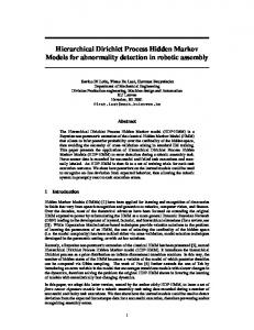
Hidden Markov Processes (HMPs) have many applications, in a wide range of disciplines - from the theory of communication [1] to analysis of gene expression [2]. Comprehensive reviews on both theory and applications of HMPs can be found in ([1], [3]). Recent applications to experimental physics are in ([4],[5]). The most widely used context of HMPs is, however, that of construction of reliable and efficient communication channels. In a practical communication channel the aim is to reliably transmit source message over a noisy channel. Fig 1. shows a schematic representation of such a communication. The source message can be a stream of words taken from a text. It is clear that such a stream of words contains information, indicating that words and letters are not chosen randomly. Rather, the probability that a particular word (or letter) appears at a given point in the stream depends on the words (letters) that were previously transmitted. Such dependency of a transmitted symbol on the precedent stream is modelled by a Markov process. The Markov model is a finite state machine that changes state once every time unit. The manner in which the state transitions occur is probabilistic and is governed by a state-transition matrix, P , that generates the new state of the system. The Markovian assumption indicates that the state at any given time depends only on the state at the previous time step. When dealing with text, a state usually represents either a letter, a word or a finite sequence of words, and the state-transition matrix represents the probability that a given state is followed by another state. Estimating the state-transition matrix is in the realm of linguistics; it is done by measuring the probability of occurrence of pairs of successive letters in a large corpus. One should bear in mind that the Markovian assumption is very restrictive and very few physical systems can expect to satisfy it in a strict manner. Clearly, a Markov process imitates some statistical properties of a given language, but can generate a chain of letters that is grammatically erroneous and lack logical meaning. Even though the Markovian description represents only some limited subset of the correlations that govern a complex process, it is the simplest natural starting point for analysis. Thus one assumes that the original message, represented by a sequence of N binary bits, has been generated by some Markov process. In the simplest scenario, of a binary symmetric Markov process, the underlying Markov model is characterized by a single parameter the flipping rate p, denoting the probability that a 0 is followed by 1 (the same as a 1 followed by a 0). The stream of N bits is transmitted through a noisy communication channel. The received string differs from the transmitted one due to the noise. The simplest way to model the noise is

2

known as the Binary Symmetric Channel, where each bit of the original message is flipped with probability ǫ. Since the observer sees only the received, noise-corrupted version of the message, and neither the original message nor the value of p that generated it are known to him, what he records is the outcome of a Hidden Markov Process. Thus, HMPs are double embedded stochastic processes; the first is the Markov process that generated the original message and the second, which does not influence the Markov process, is the noise added to the Markov chain after it has been generated. Efficient information transmission plays a central role in modern society, and takes a variety of forms, from telephone and satellite communication to storing and retrieving information on disk drives. Two central aspects of this technology are error correction and compression. For both problem areas it is of central importance to estimate ΩR , the number of (expected) received signals. In the noise free case this equals the expected number of transmitted signals ΩS ; when the Markov process has flipping rate p = 0, only two strings (all 1 or all 0) will be generated and ΩS = 2, while when the flip rate is p = 1/2 each string is equally likely and ΩS = 2N . In general, ΩR is given, for large N , by 2N H , where H = H(p, ǫ) is the entropy of the process. The importance of knowing ΩR for compression is evident: one can number the possible messages i = 1, 2, ...ΩR , and if ΩR < 2N , by transmitting only the index of the message (which can be represented by log2 ΩR < N bits) we compress the information. Note that we can get further compression using the fact that the ΩR messages do not have equal probabilities. Error correcting codes are commonly used in methods of information transmission to compensate for noise corruption of the data during transmission. These methods require the use of additional transmitted information, i.e., redundancy, together with the data itself. That is, one transmits a string of M > N bits; the percentage of additional transmitted bits required to recover the source message determines the coding efficiency, or channel capacity, a concept introduced and formulated by Shannon. The channel capacity for the BSC and for a random i.i.d. source was explicitly derived by Shannon in his seminal paper of 1948 [6]. The calculation of channel capacity for a Markovian source transmitted over a noisy channel is still an open question. Hence, calculating the entropy of a HMP is an important ingredient of progress towards deriving improved estimates of both compression and channel capacity, of both theoretical and practical importance for modern communication. In this paper we calculate the entropy of a HMP as a power series in the noise parameter ǫ. In Section 2 we map the problem onto that of a one-dimensional nearest neighbor Ising model in a field of fixed magnitude and random signs (see [7] for a review on the Random Field Ising 3

Model). Expansion in ǫ corresponds to working near the infinite field limit. Note that the object we are calculating is not the entropy of an Ising chain in a quenched random field, as shown in eq. (17) and in the discussion following it. In technical terms, here we set the replica index to n = 1 after the calculation, whereas to obtain the (quenched average) properties of an Ising chain one works in the n → 0 limit. In Sec. 3 we present exact results for the expansion coefficients of the entropy up to second order. While the zeroth and first order terms were previously known ([8], [9]), the second order term was not [10] . In Sec 4. we introduce bounds on the entropy that were derived by Cover and Thomas [11]; we have strong evidence that these bounds actually provide the exact expansion coefficients. Since we have not proved this statement, it is presented as a conjecture; on it’s basis the expansion coefficients up to eleventh order are derived and listed. We conclude in Sec. 5 by studying the radius of convergence of the low-noise expansion, and summarize our results in Sec 6.

2 2.1

A Hidden Markov Process and the Random-Field Ising Model Defining the process and its entropy

Consider the case of a binary signal generated by the source. Binary valued symbols, si = ±1 are generated and transmitted at fixed times i∆t. Denote a sequence of N transmitted symbols by S = (s1 , s2 , ....sN )

(1)

The sequence is generated by a Markov process; here we assume that the value of si+1 depends only on si (and not on the symbols generated at previous times). The process is parametrized by a transition matrix P , whose elements are the transition probabilities P+,− = P r(si+1 = +1|si = −1)

P−,+ = P r(si+1 = −1|si = +1)

Here we treat the case of a symmetric process, i.e. P+,− = P−,+ = p, si+1 =

(

si −si

prob. = 1 − p prob. = p

(2)

so that we have (3)

The first symbol s1 takes the values ±1 with equal probabilities, P r(s1 = +1) = P r(s1 = −1) = 1/2. The probability of realizing a particular sequence S is given by P r(S) =

N 1Y P r(si |si−1 ) 2 i=2

(4)

The generated sequence S is ”sent” and passes through a noisy channel; hence the received sequence, R = (r1 , r2 , ...rN ) 4

(5)

is not identical to the transmitted one. The noise can flip a transmitted symbol with probability ǫ: P r(ri = −si |si ) = ǫ

(6)

Here we assumed that the noise is generated by an independent identically distributed (iid) process; the probability of a flip at time i is independent of what happened at other times j < i and of the value of i. We also assume that the noise is symmetric, i.e. the flip probability does not depend on si . Once the underlying Markov process S has been generated, the probability of observing a particular sequence R is given by N Y

P r(R|S) =

P r(ri |si )

(7)

i=1

and the joint probability of any particular S and R to occur is given by P r(R, S) = P r(R|S)P r(S)

(8)

The original transmitted signal, S, is ”hidden” and only the received (and typically corrupted) signal R is ”seen” by the observer. Hence it is meaningful to ask - what is the probability to observe any particular received signal R? The answer is Q(R) =

X

P r(R, S)

(9)

S

Furthermore, one is interested in the1 Shannon entropy H of the observed process, HN = −

X

Q(R) log Q(R)

(10)

R

and in particular, in the entropy rate, defined as HN N →∞ N

H = lim

2.2

(11)

Casting the problem in Ising form

It is straightforward to cast the calculation of the entropy rate onto the form of a one-dimensional Ising model. The conditional Markov probabilities (3), that connect the symbols from one site to the next, can be rewritten as P r(si+1 |si ) = eJsi+1 si /(eJ + e−J ) 1

with

e2J = (1 − p)/p

The Shannon entropy is defined using log2 ; we use natural log for simplicity

5

(12)

and similarly, the flip probability generated by the noise, (6), is also recapitulated by the Ising form P r(ri |si ) = eKri si /(eK + e−K )

e2K = (1 − ǫ)/ǫ

with

(13)

The joint probability of realizing a pair of transmitted and observed sequences (S, R) takes the form ([12],[13]) P r(R, S) = A exp J

N −1 X

si+1 si + K

i=1

N X

ri s i

i=1

!

(14)

where the constant A is the product of two factors, A = A0 A1 , given by A0 =

−(N −1) 1 J e + e−J 2



A1 = eK + e−K

−N

(15)

The first sum in (14) is the Hamiltonian of a chain of Ising spins with open boundary conditions and nearest neighbor interactions J; the interactions are ferromagnetic (J > 0) for p < 1/2. The second term corresponds, for small noise ǫ < 1/2, to a strong ferromagnetic interaction K between each spin si and another spin, ri , connected to si by a ”dangling bond” (see Fig 2). Denote the summation over the hidden variables by Z(R): Z(R) =

X

exp J

S

N −1 X

si+1 si + K

i=1

N X i=1

ri si

!

(16)

so that the probability Q(R) becomes (see eq. (9)) Q(R) = A Z(R). Substituting in (10), the entropy of the process can be written as HN = −

X R

"

d X [A Z(R)]n A Z(R) log[AZ(R)] = − dn R

#

(17) n=1

The interpretation of this expression is obvious: an Ising chain is submitted to local fields hi = Kri , with the sign of the field at each site being ± with equal probabilities, and we have to average Z(h1 , ...hN )n over the field configurations. This is precisely the problem one faces in order to calculate properties of a well-studied model, of a nearest neighbor Ising chain in a quenched random field of uniform strength and random signs at the different sites (there one is interested, however, in the limit n → 0). This problem has not been solved analytically, albeit a few exactly solvable simplified versions of the model do exist ([14], [15], [16], [17]), as well as expansions (albeit in the weak field limit [18]). One should note that here we calculate the entropy associated with the observed variables R . In the Ising language this corresponds to an entropy associated with the randomly assigned signs of the local fields, and not to the entropy of the spins S. Because of this distinction the entropy

6

HN has no obvious physical interpretation or relevance, which explains why the problem has not been addressed yet by the physics community. We are interested in calculating the entropy rate in the limit of small noise, i.e. ǫ ≪ 1. In the Ising representation this limit corresponds to K ≫ 1 and hence an expansion in ǫ corresponds to expanding near the infinite field limit of the Ising chain.

3

Expansion to order ǫ2 : exact results

We are interested in calculating the entropy rate H = − lim

N →∞

"

#

1 X A Z(R) log A Z(R) N R

(18)

to a given order in ǫ. A few technical points are in order. First, we will actually use e−2K = ǫ/(1 − ǫ)

(19)

as our small parameter and expand to order ǫ2 afterwards. Second, we will calculate HN and take the large N limit. Therefore we can replace the open boundary conditions with periodic ones (setting sN +1 = s1 ) - the difference is a surface effect of order 1/N . The constant A0 becomes 

A0 = eJ + e−J

−N

(20)

and the interaction term Js1 sN is added to the first sum in eq. (14), which contains now N pairs of neighbors. Expanding Z(R): Consider Z(R) from (16). For any fixed R = (r1 , r2 , ...rN ) the leading order is obtained by the S configuration with si = ri for all i. For this configuration each site contributes K to the ”field term” in (16). The contribution of this configuration to the summation over S in (16) is (0)

Z(R)

NK

=e

exp J

N X i=1

ri+1 ri

!

(21)

The next term we add consists of the contributions of those S configurations which have si = ri at all but one position. The field term of such a configuration is K from N − 1 sites and −K from the single site with sj = −rj . There are N such configurations, and the total contribution of these terms to the sum (16) is (1)

Z(R)

N K −2K

=e

e

exp J

N X

ri+1 ri

i=1

7

!

N X

j=1

exp[−2Jrj (rj−1 + rj+1 )]

(22)

The next term is of the highest order studied in this paper; it involves configurations S with all but two spins in the state si = ri ; the other two take the values sj = −rj , sk = −rk , i.e. are flipped with respect to the corresponding local fields. These S configurations belong to one of two classes. In class a the two flipped spins are located on nearest neighbor sites, e.g. k = j + 1; there are N such configurations. To the second class, b, belong those configurations in which the two flipped spins are not neighbors - there are N (N − 3)/2 such terms in the sum (16), and the respective contributions are2 (2a)

Z(R)

N K −4K

=e

e

exp J

N X

ri+1 ri

i=1

Z(R)(2b) = eN K e−4K exp J

N X

ri+1 ri

i=1

!

!

N X

exp[−2J(rj rj−1 + rj+1 rj+2 )]

(23)

j=1

N X 1X exp[−2Jrj (rj−1 + rj+1 ) − 2Jrk (rk−1 + rk+1 )] 2 j=1 k6=j,j±1

(24)

Calculation of H is now straightforward, albeit tedious: substitute AZ into eq. (18), expand everything in powers of ǫ, to second order, and for each term perform the summation over all the ri variables. These summations involve two kinds of terms. The first is of the ”partition-sum-like” form X

eH(R)

where

H(R) =

X

∆j Jrj rj+1

with

∆j = ±1

(25)

j

R

For the case studied here we encounter either all bonds ∆j J > 0, or two have a flipped sign (corresponding to eq. (22, 23)), or four have flipped signs (corresponding to (24)). These ”partitionsum-like” terms are independent of the signs of the ∆j ; in fact we have for all of them A0

X

eH(R) = 1

(26)

R

The second type of term that contributes to H is of the ”energy-like” form: X

eH(R) rk rk+1

(27)

R

The absolute value of these terms is again independent of the ∆j , but one has to keep track of their signs. Finally, one has to remember that the constant A1 also has to be expanded in ǫ. The calculation finally yields the following result (here we switch from J to the ”natural” variable p using eq. (12)): H(p, ǫ) =

∞ X

H (k) (p)ǫk

k=0 2

We use the obvious identifications imposed by periodic boundary conditions, e.g. rN+1 = r1 , rN+2 = r2

8

(28)

with the coefficients Hk given by : H

(0)

= −p log p − (1 − p) log(1 − p) H

(2)

H

(1)

1−p = 2(1 − 2p) log p 



1−p (1 − 2p)2 = −2(1 − 2p) log − 2 p 2p (1 − p)2 



(29) (30)

The zeroth and first order terms (29) were known ([8], [9]), while the second order term is new [10].

4

Upper Bounds derived using a system of finite length

When investigating the limit H, it is useful to study the quantity CN = HN − HN −1 , which is also known as the conditional entropy. CN can be interpreted as the average amount of uncertainty we have on rN , assuming that we know (r1 , . . . , rN −1 ). Provided that H exist, it easily follows that H = lim CN

(31)

N →∞

Moreover, according to [11], CN ≥ H, and the convergence is monotone : CN ց H

(N → ∞)

(32)

We can express CN as a function of p and ǫ by using eq. (17). For this, we represent Z using the original variables p, ǫ (note that from this point of we work with open boundary conditions on the Ising chain of N spins):

Z(R) =

X

PN−1

(1 − p)

S

i=1

1Si =Si+1 N −1−

p

PN−1 i=1

1Si =Si+1

PN

(1 − ǫ)

i=1

1Si =Ri N −

ǫ

Pn

i=1

1Si =Ri

(33)

where we denote 1s,s′ = (1 + ss′ )/2. Eq. (33) gives Z(R) explicitly as a polynomial in p and ǫ with maximal degree N , and can be represented as :

Z(R) =

N X

Zi (R)ǫi

(34)

i=0

Here Zi = Zi (R) are functions of p only. Substituting this expansion in eq. (17), and expanding log Z(R) according to the Taylor series log(a + x) = log(a) −

HN = −

(−x)n n=1 nan ,

P∞

"N X X R

i=0

we get

Zi (R)ǫi

#"

log Z0 (R)−

k X (−

j=1

9

Pn



i j i=1 Zi (R)ǫ )  + O(ǫk+1 ) jZ0 (R)j

(35)

When extended to terms of order ǫk , this equation gives us precisely the expansion of the upperbound CN up to the k-th order, CN =

k X

(i)

CN ǫi + O(ǫk+1 )

(36)

i=0

For example, stopping at order L = 2 gives HN = −

X

Z0 (R) log Z0 (R)+ [Z1 (R)(1 + log Z0 (R))] ǫ+

Y

"

#

Z1 (R)2 + Z2 (R)(1 + log Z0 (R)) ǫ2 2Z0 (R)

)

+ O(ǫ3 )

(37)

The zeroth and first order terms can be evaluated analytically for any N ; beyond first order, we can compute the expansion of HN symbolically 3 (using Maple [19]), for any finite N . This was actually (1)

done, for N ≤ 8 and k ≤ 11. For the first order we have proved ([10]) that CN is independent of N (and equals H (1) ). The symbolic computation of higher order terms yielded similar independence (2)

(k)

of N , provided that N is large enough. So, CN = C (k) for large enough N . For example, CN is independent of N for 3 ≤ N ≤ 8 and equals the exact value of H (2) as given by eq. (30). Similarly, (4)

CN settles, for N ≥ 4, at some value denote by C (4) , and so on. For the values we have checked, (k)

the settling point for CN turned out to be at N = ⌈ k+3 2 ⌉. This behavior is, however, unproved for k ≥ 2, and, therefore, we refer to it as a Conjecture: For any order k, there is a critical chain length Nc (k) = ⌈ k+3 2 ⌉ such that for (k)

N > Nc (k) we have CN = C (k) . It is known that CN → H, and CN and H are analytic functions of ǫ at ǫ = 0 4 , so that we (k)

can expand both sides around ǫ = 0, and conclude that CN → H (k) for any k ≥ 1 when N → ∞. (k)

Therefore, if our conjecture is true, and CN indeed settles at some value C (k) independent of N (for N > Nc (k) ), it immediately follows that this value equals H (k) . Note that the settling is rigourously supported for k = 0, 1, while for k = 2 we showed that indeed C (2) = H (2) , supporting our conjecture. The first orders up to H (11) , obtained by identifying H (k) with C (k) , are given in the Appendix, as functions of λ = 1 − 2p, for better readability. The values of H (0) , H (1) and H (2) coincide with the results that were derived rigorously from the low-temperature/high-field expansion, thus giving us support for postulating the above Conjecture. 3 4

The computation we have done is exponential in N , but the complexity can be improved. See next section on the Radius of Convergence

10

Interestingly, the nominators have a simpler expression when considered as a functions of λ, which is the second eigenvalue of the Markov transition matrix P . Note that only even powers of λ appear. Another interesting observation is that the free element in [p(1 − p)]2(k−1) H (k) (when treated as a polynomial in p), is

(−1)k k(k−1) ,

ǫ which might suggest some role for the function log(1 + [2p(1−p)] 2 ) in the

first derivative of H. All of the above observations led us to conjecture the following form for H (k) (for k ≥ 3) : H

(k)

=

k(k −

Pdk

2j j=0 aj,k λ 1)(1 − λ2 )2(k−1)

24(k−1)

(38)

where aj,k and dk are integers that can be seen in the Appendix for H (k) up to k = 11.

5

The Radius of Convergence

If one wants to use our expansion around ǫ = 0 for actually estimating H at some value ǫ, it is important to ascertain that ǫ lies within the radius of convergence of the expansion. The fundamental observation made here is that for p = 0, the function H(ǫ) is not an analytic function at ǫ = 0, since its first derivative diverges. As we increase p, the singularity points ’moves’ to negative values of ǫ, and hence the function is analytic at ǫ = 0, but the radius of convergence is determined by the distance of ǫ = 0 from this singularity. Denote by ρ(p) the radius of convergence of H(ǫ) for a given p; we expect that ρ(p) grows when we increase p, while for p → 0, ρ(p) → 0. It is useful to first look at a simpler model, in which there is no interaction between the spins. Instead, each spin is in an external field which has a uniform constant component J, and a sitedependent component of absolute value K and a random sign. For this simple i.i.d. model the entropy rate takes the form H = hb [p(1 − ǫ) + ǫ(1 − p)]

(39)

where hb [x] = −[x log x + (1 − x) log(1 − x)] is the binary entropy function. Note that for ǫ = 0 the entropy of this model equals that of the Ising chain. Expanding eq. (39) in ǫ (for p > 0) gives : H = −(p log p + (1 − p) log(1 − p)) + (1 − 2p) log( ∞ X

#

"

1 (1 − 2p)k (2p − 1)k + ǫk k k−1 k(k − 1) p (1 − p) k=2

1−p )ǫ+ p (40)

The radius of convergence here is easily shown to be p/(1 − 2p); it goes to 0 for p → 0 and increases monotonically with p. Returning to the HMP, the orders H (k) are (in absolute value) usually larger than those of the simpler i.i.d. model, and hence the radius of convergence may be expected to be smaller. Since we 11

could not derive ρ(p) analytically, we estimated it using extrapolation based on the first 11 orders. We use the fact that ρ(p) = limk→∞

H (k) H (k+1)

(provided the limit exists). The data was fitted to a

rational function of the following form (which holds for the i.i.d. model): H (k) ak + b ∼ , (k+1) k+c H

(41)

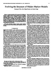
For a given fit, the radius of convergence was simply estimated by a. The resulting prediction is given in Fig. 3 for both the i.i.d. model (for which it is compared to the known exact ρ(p)) and for the HMP. While quantitatively, the predicted radius of the HMP is much smaller than this of the i.i.d. model, it has the same qualitative behavior, of starting at zero for p = 0, and increasing with p. We compared the analytic expansion to estimates of the entropy rate based on the lower and upper bounds, for two values of ǫ (see Fig. 4) . First we took ǫ = 0.01, which is realistic in typical communication applications. For p less than about 0.1 this value of ǫ exceeds the radius of convergence and the series expansion diverges, whereas for larger p the series converges and gives a very good approximation to H(p, ǫ = 0.01). The second value used was ǫ = 0.2; here the divergence happens for p ≤ 0.37, so the expansion yields a good approximation for a much smaller range. We note that, as expected, the approximation is much closer to the upper bound than to the lower bound of [11].

6

Summary

Transmission of a binary message through a noisy channel is modelled by a Hidden Markov Process. We mapped the binary symmetric HMP onto an Ising chain in a random external field in thermal equilibrium. Using a low-temperature/high-random-field expansion we calculated the entropy of the HMP to second order k = 2 in the noise parameter ǫ. We have shown for k ≤ 11 that when the known upper bound on the entropy rate is expanded in ǫ, using finite chains of length N , the expansion coefficients settle, for Nc (k) ≤ N ≤ 8, to values that are independent of N . Posing a conjecture, that this continues to hold for any N , we identified the expansion coefficients of the entropy up to order 11. The radius of convergence of the resulting series was studied and the expansion was compared to the the known upper and lower bounds. By using methods of Statistical Physics we were able to address a problem of considerable current interest in the problem area of noisy communication channels and data compression.

12

Acknowledgments I.K. thanks N. Merhav for very helpful comments, and the Einstein Center for Theoretical Physics for partial support. This work was partially supported by grants from the Minerva Foundation and by the European Community’s Human Potential Programme under contract HPRN-CT-200200319, STIPCO.

References [1] Y. Ephraim and N. Merhav, ”Hidden Markov processes”, IEEE Trans. Inform. Theory, vol. 48, p. 1518-1569, June 2002. [2] A. Schliep, A. Sch¨ onhuth and C. Steinhoff, ”Using hidden Markov models to analyze gene expression time course data”, Bioinformatics, 19, Suppl. 1 p. i255-i263, 2003. [3] L. R. Rabiner, ”A tutorial on hidden Markov models and selected applications in speech recognition”, Proc. IEEE, vol. 77, p. 257286, Feb 1989. [4] I. Kanter, A. Frydman and A. Ater, ”Is a multiple excitation of a single atom equivalent to a single ensemble of atoms?” Europhys. Lett., 2005 (in press). [5] I. Kanter, A. Frydman and A. Ater, ”Utilizing hidden Markov processes as a new tool for experimental physics”, Europhys. Lett., 2005 (in press). [6] C. E. Shannon, ”A mathematical theory of communication”, Bell System Technical Journal, 27, p. 379-423 and 623-656, Jul and Oct, 1948. [7] T. Nattermann, ”Theory of the Random Field Ising Model”, in Spin Glasses and Random Fields, ed. by A.P. Young, World Scientific 1997. [8] P. Jacquet, G. Seroussi and W. Szpankowski, ”On the Entropy of a Hidden Markov Process”, Data Compression Conference , Snowbird, 2004. [9] E. Ordentlich and T. Weissman, ”New Bounds on the Entropy Rate of Hidden Markov Processes”, San Antonio Information Theory Workshop, Oct 2004. [10] A preliminary presentation of our results is given in O. Zuk, I. Kanter and E. Domany, ”Asymptotics of the Entropy Rate for a Hidden Markov Process”, Data Compression Conference , Snowbird, 2005. [11] T. M. Cover and J. A. Thomas, ”Elements of Information Theory”, Wiley, New York, 1991. [12] L. K. Saul and M. I. Jordan, ”Boltzmann chains and hidden Markov models”, Advances in Neural Information Processing Systems 7, MIT Press, 1994. [13] D. J.C. MacKay, ”Equivalence of Boltzmann Chains and Hidden Markov Models”, Neural Computation, vol. 8 (1), p. 178-181, Jan 1996. 13

[14] B. Derrida, M.M. France and J. Peyriere, ”Exactly Solvable One-Simensional Inhomogeneous Models”, Journal of Stat. Phys. 45 (3-4), p. 439-449, Nov 1986. [15] D.S. Fisher , P. Le Doussal and P. Monthus, ”Nonequilibrium dynamics of random field Ising spin chains: Exact results via real space renormalization group” Phys. Rev. E, 64 (6), p. 066-107, Dec 2001. [16] G. Grinstein and D. Mukamel, ”Exact Solution of a One Dimensional Ising-Model in a Random Magnetic Field”, Phys. Rev. B, 27, p. 4503-4506, 1983. [17] T. M. Nieuwenhuizen and J.M. Luck, ”Exactly soluble random field Ising models in one dimension”, J. Phys. A: Math. Gen., 19 p. 1207-1227, May 1986. [18] B. Derrida and H. J. Hilhorst, J. Phys. A 16 2641 (1983) [19] http://www.maplesoft.com/

Appendix Orders three to eleven, as function of λ = 1 − 2p. (Orders 0 − 2 are given in equations (29 - 30)) : H (3) =

H (4) =

H (5) =

−16(5λ4 − 10λ2 − 3)λ2 3(1 − λ2 )4

8(109λ8 + 20λ6 − 114λ4 − 140λ2 − 3)λ2 3(1 − λ2 )6

−128(95λ10 + 336λ8 + 762λ6 − 708λ4 − 769λ2 − 100)λ4 15(1 − λ2 )8

H (6) = 128(125λ14 − 321λ12 + 9525λ10 + 16511λ8 − 7825λ6 − 17995λ4 − 4001λ2 − 115)λ4 /15(1 − λ2 )10

H (7) = −256(280λ18 − 45941λ16 − 110888λ14 + 666580λ12 + 1628568λ10 − 270014λ8 − 1470296λ6 − 524588λ4 − 37296λ2 − 245)λ4 /105(1 − λ2 )12

H (8) = 64(56λ22 − 169169λ20 − 2072958λ18 − 5222301λ16 + 12116328λ14 + 14

35666574λ12 + 3658284λ10 − 29072946λ8 − 14556080λ6 − 1872317λ4 − 48286λ2 − 49)λ4 /21(1 − λ2 )14

H (9) = 2048(37527λ22 + 968829λ20 + 8819501λ18 + 20135431λ16 − 23482698λ14 − 97554574λ12 − 30319318λ10 + 67137630λ8 + 46641379λ6 + 8950625λ4 + 495993λ2 + 4683)λ6 /63(1 − λ2 )16

H (10) = −2048(38757λ26 + 1394199λ24 + 31894966λ22 + 243826482λ20 + 571835031λ18 − 326987427λ16 − 2068579420λ14 − 1054659252λ12 + 1173787011λ10 + 1120170657λ8 + 296483526λ6 + 26886370λ4 + 684129λ2 + 2187)λ6 /45(1 − λ2 )18

H (11) = 8192(98142λ30 − 1899975λ28 + 92425520λ26 + 3095961215λ24 + 25070557898λ22 + 59810870313λ20 − 11635283900λ18 − 173686662185λ16 − 120533821070λ14 + 74948247123λ12 + 102982107048λ10 + 35567469125λ8 + 4673872550λ6 + 217466315λ4 + 2569380λ2 + 2277)λ6 /495(1 − λ2 )20

15

Figure 1: Schematic drawing of message transmission through a noisy channel.

16

Figure 2: An Ising model in a random field. The solid lines represent interactions of strength J between neighboring spins Si while the dashed lines represent local fields Kri acting on the spin Si .

17

1.6

Radius of Convergence

1.4

True Radius Predicted Radius HMM Predicted Radius

1.2 1 0.8 0.6 0.4 0.2 0 0.05

0.1

0.15

0.2

0.25

0.3

0.35

0.4

P

Figure 3: Radius of convergence for the i.i.d. model (estimated and exact, see text), and HMP (estimated) for 0.05 ≤ p ≤ 0.35.

18

ε = 0.01

ε = 0.2

1

Entropy Estimation

Entropy Estimation

0.9

0.8

0.7

0.6

0.5

0.4

Expansion Upper Bound Lower Bound

1.03

Expansion Upper Bound Lower Bound

1.02

1.01

1

0.99

0.98

0.1

0.15

0.97

0.2

p

0.35

0.4

0.45

0.5

p

Figure 4: Approximation using the first eleven orders in the expansion, for ǫ = 0.01 (left) and ǫ = 0.2 (right), for various values of p. For comparison, upper and lower bounds (using N = 2 from [11]) are displayed. For each ǫ there is some critical p below which the series diverges and the approximation is poor. For larger p the approximation becomes better.

19