The equivalence between the operator approach and the path integral ...

arXiv:hep-th/9511141v1 20 Nov 1995

ITP-SB-95-49 QMW-PH-95-40

The equivalence between the operator approach and the path integral approach for quantum mechanical non-linear sigma models1 Jan de Boer, Bas Peeters, Kostas Skenderis, and Peter van Nieuwenhuizen Institute for Theoretical Physics, State University of New York at Stony Brook Stony Brook, NY 11794-3840, U.S.A.

Abstract: We give background material and some details of calculations for two recent papers [1,2] where we derived a path integral representation of the transition element for supersymmetric and nonsupersymmetric nonlinear sigma models in one dimension (quantum mechanics). Our approach starts from a Hamiltonian ˆ ψˆ† ) with a priori operator ordering. By inserting a finite number of comH(ˆ x, pˆ, ψ, plete sets of x eigenstates, p eigenstates and fermionic coherent states, we obtain the discretized path integral and the discretized propagators and vertices in closed form. Taking the continuum limit we read off the Feynman rules and measure of the continuum theory which differ from those often assumed. In particular, mode regularization of the continuum theory is shown in an example to give incorrect results. As a consequence of time-slicing, the action and Feynman rules, although without any ambiguities, are necessarily noncovariant, but the final results are covariant if ˆ is covariant. All our derivations are exact. Two loop calculations confirm our H results.

1

Introduction.

The subject of path integrals in curved space is arcane, complicated and controversial [3]. In two recent articles we have considered one-dimensional (quantum mechanical) path integrals, and found an exact path integral representation for the transition element [1,2]. For the bosonic case it is defined by T (z, y; β) = ˆ x, pˆ)|y > where |y > and < z| are position eigenstates. The classical < z| exp − β H(ˆ h ¯

1

to appear in proceedings of workshop on gauge theories, applied supersymmetry and quantum gravity, Leuven, Belgium, July 10-14, 1995, and strings’95, USC, March 13-18, 1995.

Lagrangian is given by Lcl = 21 gij (x)x˙ i x˙ j , but both the quantum Hamiltonian and the action in the path integral deviate substantially from Lcl . We begin by assuming ˆ has a given a priori operator ordering. By inserting N − 1 complete sets of that H

x eigenstates and N sets of p eigenstates, one finds a discretized phase space path integral, from which one can derive (as we shall indeed do) discretized propagators and vertices in closed form (by coupling to discretized external sources). In the continuum limit one obtains then a Euclidean path integral of the form Z

R0

dp dx e

(ipq−H(p,q)}dt ˙

−β

(1)

with well-defined propagators, vertices, and rules how to evaluate Feynman graphs. The last result is the most important: these rules are new and differ from what is usually assumed. If one would bypass a detailed analysis of the discretized case, one might expect ˆ is a covariant operator. (For example, that L = ipq˙ − H(p, q) is covariant if H ˆ would commute with the supersymmetry generators, one might expect that if H after integrating out p, the resulting actions are the supersymmetric actions one encounters in the literature). This is incorrect: the action needs noncovariant terms of order h ¯ and h ¯ 2 (but not beyond) in order that T be covariant. Another source of puzzlement might be the observation that actions of the form L = 12 gij (x)x˙ i x˙ j contain double-derivative interactions, leading to linearly divergent graphs by power counting. On the other hand, it is well-known that quantum mechanics is a finite theory. It would seem strange (and is, in fact, incorrect) to require that normal-ordering removes divergences: where would normal ordering come from? The resolution of this paradox will be the presence of new ghosts, closely related to the factors g 1/2 δ(0) which Lee and Yang found in a careful treatment of the deformed harmonic oscillator [4], and which we shall call for this reason “LeeYang ghosts”. (They were first introduced by Bastianelli, and in a more covariant form by him and one of us [5]). The propagator for the quantum deviations of a scalar q(τ ) (where τ = t/β) on the interval (−1, 0) with boundary conditions q(−1) = q(0) = 0 is proportional to 1 1 ∆(σ, τ ) = ∆F (σ − τ ) + (στ + σ + τ ) 2 2

(2)

where ∆F (σ −τ ) = 21 (σ −τ )θ(σ −τ )+ 12 (τ −σ)θ(τ −σ) is the translationally invariant

solution of ∂σ2 ∆F (σ−τ ) = δ(σ−τ ) while the terms στ + 21 σ+ 12 τ enforce the boundary conditions. In Feynman graphs, contractions between x and x, ˙ and between x˙ and 2

x, ˙ produce θ(σ − τ ) and δ(σ − τ ), and the problem arises how to evaluate products of several δ(σ − τ ) and θ(σ − τ ). Mathematically, various consistent but different

definitions of these products of distributions can be given [6], but physically (1) should have an unambiguous meaning, and the problem is to find the correct rules. Consider as an example Z

0

−1

Z

0

−1

δ(σ − τ )θ(σ − τ )θ(σ − τ )dσdτ

(3)

One might expect that, since δ(σ − τ ) = ∂σ θ(σ − τ ), the result is equal to 1 R0 R0 ∂ [θ(σ − τ )3 ]dσdt = 13 . However, the correct result is 14 as the discretized 3 −1 −1 σ approach shows.

Another source of ambiguities are the equal-time contractions, in particular < x(τ ˙ )x(τ ˙ ) >. Are these the limit of < x(τ ˙ 1 )x(τ ˙ 2 ) > for τ1 → τ2 , and what to do with the resulting δ(0)? In field theory, equal-time contractions are a priori undefined, and one needs a symmetry principle to fix them, but here everything has been specified from the beginning, so ambiguities in equal-time contractions are not allowed. Yet another worry would be the perennial headache called “the measure”. Since the path integrals correspond to a one-dimensional quantum field theory on a finite time segment, one might expect some factors in the measure to be present, like det g to some power at the end points. In fact, in Hamiltonian quantization of gravity in higher dimensions, such factors (and factors involving g00 ) are present. We shall see that also in our case there are nontrivial measure factors. These are usually omitted in calculations with nonlinear sigma models, but are crucial to obtain the correct results. What do we exactly mean by “correct results”? “Correct results” means for ˆ >, no more and no less. This us: the results which agree with < z| exp − β¯h H|y matrix element can be straightforwardly evaluated order by order in β, without encountering any divergences or ambiguities, simply by expanding the exponent and inserting a complete set of p-states T (z, y; β) =

Z

β ˆ | p >< p|y > d4 p < z| exp − H h ¯

(4)

Moving all xˆj to the left and all pˆj to the right, keeping track of commutators, one obtains c-number results. All terms with a given number of commutators, say s, are of a given order in β (see below), and although for each s an infinite number of terms contributes, one can sum the infinite series for fixed s in closed form. Thus 3

T (z, y; β) is a finite and unambiguous Laurent series in β. Our task is to find a path integral which reproduces these terms order by order in loops (in the path integral, β and h ¯ appear only in the combination β¯ h, so β also counts the number of loops on the worldline). One could, of course, reject this Hamiltonian starting point, and try to devise a more covariant way of defining path integrals in curved space which does ˆ x, pˆ). In particular, whereas in our approach not require a given Hamiltonian H(ˆ we encounter noncovariant “midpoint rules” like x¯k+1/2 = 21 (xk+1 + xk ), one might hope that covariant midpoint rules (the middle of a geodesic, for example) might lead to a completely covariant treatment. All we can say is that we have found a path integral which yields the correct results and which straightforwardly follows from T (z, y; β) by inserting complete sets of states, whereas the more covariant approaches have so far not been able to reach the same results2 . There are good practical reasons for starting with the Hamiltonian matrix element < z| exp −β/¯ hH|y >, rather than a covariant configuration space starting point. When one calculates anomalies in n-dimensional quantum field theories, one can rewrite these anomalies as products of matrix elements of the Jacobian times T [7], Z q q β g(y) < y|J|z > g(z) < z| exp − H|y > dn ydn z An = (5) h ¯

The extension to include fermions is straightforward. So, quantum mechanics enters via T , and the reason one wants to rewrite T as a path integral is that the calculations of anomalies are much simpler in the path integral approach than in the Hamiltonian approach. We shall not discuss these applications to anomalies here, but refer to [2]. We shall also not discuss fermions in detail here (again, see [2]), but only say that one can introduce bras and kets |η > and < η¯| which are eigenstates of the fermionic annihilation and absorption operators ψˆa and ψˆa† , respectively. These states are coherent states |η >= (exp ψa† η a )|0 > and < η¯| =< 0| exp η¯a ψ a with η a and η¯a independent Grassmann variables (so not related by complex conjugation, 2

Covariant techniques to evaluate path integrals do exist, but can only be used when the path integral has additional special properties, for example if the semi-classical approximation is exact, or if the theory has additional symmetries so that one can use localization techniques. However, such techniques do not extend to arbitrary path integrals. In order to set up perturbation theory, one has to choose a decomposition S = S (0) + S int , and in the case of a general σ model it is not true that S (0) and S int can be chosen to be separately covariant. (The kinetic operator in the full quadratic term is covariant, but not invertible in closed form[3].) Thus, Feynman rules based purely on S (0) are necessarily noncovariant.

4

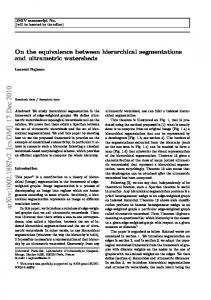
Schrodinger equation for heat kernel (DeWitt)

〈 z | exp - β-h H | y 〉

final result direct operator methods

Weyl ‘‘Trotter’’ Berezin loops

discrete phase space path integral

new ghosts

discrete configuration space path integral

subtle

continuous phase space path integral

Matthews new ghosts

continuous configuration space path integral

no products of distributions, no subtleties

R

only satisfying dηη =

R

d¯ ηη¯ = 1). This is the fermionic equivalent of the “holomor-

phic” representation for bosonic systems [8]. We have found it simplest to use the x, p representation for coordinates, but for the fermionic part the ψ, ψ † representation is by far the most natural. (One could, however, also construct a kind of x, p representation for the fermions). The fermionic coherent states satisfy completeness relations and for N = 2 supersymmetric systems there is really no major obstacle √ to construct T (¯ η, z, η, y; β): one combines ψαa (α = 1, 2) into ψ a ≡ (ψ1a + iψ2a )/ 2 and √ ψa† = (ψ1a − iψ a )/ 2. However, for N = 1 supersymmetric systems, one has n Majorana fermions ψˆa (a = 1, . . . , n) satisfying the Dirac brackets {ψˆa , ψˆb } = δ ab . To construct a vacuum and coherent states, we need rather ψ A and ψA† satisfying ψ A |0 >= 0, {ψ A , ψ B } = 0, {ψA† , ψB† } = 0 and {ψ A , ψB† } = δ A B . This can be achieved in two ways: a (i) by fermion doubling, namely adding a second set of free fermions ψII which do not

appear in the Hamiltonian but which are used to construct ψ A and ψA† as ψ A = (ψIa + √ √ a a iψII )/ 2 and ψA† = (ψIa − iψII )/ 2. Here ψIa denotes the original set of fermions ψ a .

(ii) by fermion halving, namely as follows √ √ ψ A = (ψ 2A−1 + iψ 2A )/ 2, ψA† = (ψ 2A−1 − iψ 2A )/ 2

(6)

The vacuum and Hilbert space are different in both cases, and one finds different results for the propagators and transition elements (!), but the anomalies come out the same. This is as expected: in traces over Hilbert space, differences created by choosing different vacua should cancel. In the next sections we shall give some details of calculations which are only 5

briefly summarized in [1,2]. A flow chart of the main ideas is given above.

2

Weyl ordering and an extension of the Trotter formula.

ˆ E which plays a role For definiteness one may consider a particular Hamiltonian H in the calculation of anomalies ˆ E = 1 g −1/4 pi g 1/2 g ij pj g −1/4 H 2

(7)

This operator is Einstein invariant, but we stress that our results hold for any other operator with two p’s. Inserting (N − 1) complete sets of x eigenstates and N comq

plete sets of p eigenstates, using the completeness relations |x > g(x) < x|dn x = R |p >< p|dn p = I, we find an expression for T (z, y; β) in terms of N kernels R

T (xk , xk−1 ; ǫ) =

Z

ǫ ˆ n < xk | exp − H|p k >< pk |xk−1 > d pk , h ¯

(8)

ˆ as a Weyl ordered operator. For where xN = z, x0 = y and ǫ = β/N. We rewrite H a polynomial in p’s and x’s, the corresponding Weyl ordered operator is obtained by expanding (αj pˆj + βi xˆi )N and retaining all terms with a particular combination of α’s and β’s. It follows that (g ij pi pj )W = 41 pˆi pˆj gˆij + 21 pˆi gˆij pˆj + 41 gˆij pˆi pˆj , and by ˆ − ( 1 g ij pi pj )W one finds extra terms of order h ¯2 evaluating H 2 ¯ 2 ℓ k ij ˆ = 1 (g ij pi pj )W + h (Γ Γ g + R) H 2 8 ik jℓ

(9)

ˆ in which the p’s appear less symmetrically (on a sphere R < 0). Other operators H will in general also lead to ¯ . For a polynomial one may prove  terms of order h  extra m  m−ℓ r ℓ P  that (xm pr )W = 21m m xˆ pˆ xˆ , and it follows that ℓ=0 ℓ m X





1  m  Z m−ℓ r ℓ < z|(x p )W |y > = z p y < z|p >< p|y > dn p m ℓ ℓ=0 2   Z z+y m r p < p|y > dn p = < z|p > 2 m r

(10)

This shows why orderings like Weyl ordering are very convenient: one can replace a Weyl ordered operator by a function, simply by substituting pˆ → p, xˆ → 12 (z + y), and this is an exact result. 6

However, Weyl ordering and exponentiation do not commute, (exp − ¯hǫ H)W 6= exp − ¯hǫ (HW ), and whereas HW was easy to write down, a closed expression for

(exp − ¯hǫ H)W cannot be written down. One expects, however, that a suitable approximation of the kernels, containing only terms of order ǫ suffices. Here one stumbles upon a problem: it might seem that p is of order ǫ−1/2 due to the term exp − 21 ǫp2 in the action. Expansion of exp − ¯hǫ HW would contain terms of the form ǫs pr f (x) for which s ≥ 2 but which would still be of order ǫ. We are now going to

give an argument that p is of order unity, and therefore only the terms with one explicit ǫ need be retained. Hence, we will use as kernel exp − ¯hǫ HW ( 12 (xk +xk−1 ), pk ).

In other words, the Trotter-like approximation

ǫ ˆ ǫ ǫ ǫ ˆ >≃< x|1 − H|p >= (1 − h) < x|p >=< x|p > exp − h (11) < x| exp − H|p h ¯ h ¯ h ¯ h ¯ ˆ > as in the usual models with H = is still correct, but h is not simply < x|H|p T (p) + V (x), but rather it equals HW at the midpoints. To obtain this result, we note that the kernels are exactly equal to Z

n

d pk e

i ~ k−1/2 p ~ ·∆x h ¯ k



ǫ −h H ¯

e



W

(¯ xk−1/2 , pk );

∆xk−1/2 = xk − xk−1 x¯k−1/2 = 21 (xk + xk−1 )

(12)

The difference between (exp − ¯hǫ H)W and exp − ¯hǫ (HW ) consists of two kinds of terms (i) terms without a p ; these are certainly of higher order in ǫ and can be omitted (ii) terms with at least one p. The crucial observation [9] is now that the phase space propagators < pk,i pl,j > and < pk,ix¯jk+1/2 > are both of order unity, and not of order ǫ−1 and ǫ−1/2 , respectively. A formal proof is given in equation (35). However, already at this point one might note that the pp propagator is not only determined by the gpp term but also by ip∆q. Completing squares, it is the p′ = (p − i∆q/ǫ) which is of order ǫ−1/2 . In the pp propagator the singularities of the p′ p′ and ∆q∆q propagators cancel each other. As a consequence, the pp and p¯ q propagators are of order one, and this proves the Trotter formula also for nonlinear sigma models. The final result is that one may use exp − ¯hǫ HW ( 12 (xk +xk−1 ), pk ) as the kernels of

the path integral. If one would not have used Weyl ordering, but simply computed R ˆ k >< pk |xk−1 > dn pk keeping all terms of order ǫ, one finds terms < xk | exp − ¯hǫ H|p proportional to Rij (¯ xk−1/2 )∆xik−1/2 ∆xjk−1/2 where Rij is the Ricci tensor. These R terms do not correspond to a local action (they are of the form Rij x˙ i x˙ j dtǫ). These 7

nonlocal kernels will yield the correct answer for the path integral, but Feynman rules for nonlocal theories are a headache, and it is not clear whether a truncation of these kernels to a local action exists which yields the correct answer. Weyl ordering, on the other hand, does lead to local kernels which are very easy to construct and which yield the correct result. This demonstrates the usefulness of Weyl ordering.

3

Discretized propagators and new Feynman rules.

If we keep the pk,j and xjk as integration variables we obtain a discretized phase space path integral, but if we integrate the pk,j out, we get a discretized configuration space path integral with N factors [det gij (¯ xk+1/2 )]1/2 . In the continuum limit Lee and Yang wrote these determinants as exp 12 δ(0)tr ln gij dt and treated the exponent as a new term in the action [4]. We first discuss these configuration space path integrals. For the same calculational advantages as in the case of Faddeev-Popov ghosts in gauge theories, we exponentiate these determinants by ghosts, but whereas the Faddeev-Popov determinant needs a pair of anticommuting real ghosts/antighosts, here the square root of the determinant requires an extra third commuting real ghosts. One obtains then the following path integral [5] NY −1

(det gij (¯ xk+1/2 ))1/2 =

k=0

α

Z

i h 1 xk+1/2 ) bik+1/2 cjk+1/2 + aik+1/2 ajk+1/2 (13) dbk+1/2 dck+1/2 dak+1/2 exp gij (¯ 2

where α is a constant which can easily be determined. We decompose the xk into a sum of background parts and quantum parts, xjk = xjbg,k + qkj , and the action S into a free part S (0) =

N −1 X k=0

  1 j i gij (z) ∆qk+1/2 ∆qk+1/2 + bik+1/2 cjk+1/2 + aik+1/2 ajk+1/2 2

(14)

and an interaction part S int (the rest), requiring that the background fields satisfy the (discretized) equation of motion of S (0) and the boundary conditions. Hence qN = q0 = 0. With the continuum limit in mind we parametrize the discrete qk using continuum modes of S (0) qkj

=

N −1 X m=1

r

j

m

s

kmπ 2 sin ; k = 1, . . . , N − 1 N N 8

(15)

j j to and q¯k+1/2 The Jacobian for xk → qk → rm is unity. We then couple ∆qk+1/2 discretized external sources

S(sources) = −

N −1 X

j j (Fk+1/2,j ∆qk+1/2 + ǫGk+1/2, q¯k+1/2 ).

(16)

k=0

Similarly we introduce discretized sources for the ghosts b, c and a. We then complete squares and integrate over the discrete variables rm j , bj k+1/2 , cj k+1/2 , aj k+1/2 . The result is a functional quadratic in external sources which will yield the discretized propagators. We first quote the result and then give details of the calculation. By differentiating twice w.r.t G one finds 1 1 1 j i < q¯k+1/2 q¯ℓ+1/2 >= ǫ¯ hg ij (z) −(k + )(ℓ + )/N + (ℓ + )θk,ℓ + (k + 1/2)θℓ,k 2 2 2 

where θk,ℓ is the discretized θ function (θk,ℓ = 0 if k < ℓ, θk,ℓ =

1 2



(17)

if k = ℓ and θk,ℓ = 1

if k > ℓ). In the continuum limit this becomes k + 12 −1 = −β¯ hg ij (z)∆(σ, τ ) ; −1 < σ =

(18)

Similarly i

< q¯ k+1/2 ∆q

j

ℓ+1/2

< ∆q i k+1/2 ∆q j ℓ+1/2 < bi k+1/2 cj ℓ+1/2

k + 12 + θk,ℓ > = ǫ¯ hg (z) − N ǫ¯ h ij > = g (z) [−1 + Nδk,ℓ ] N 1 ij 2 ij ¯ g (z)δk,ℓ ; < ai k+1/2 aj ℓ+1/2 >= h ¯ g (z)δk,ℓ (19) > = − h ǫ ǫ ij

"

#

These results show that in the continuum limit θ(σ − τ ) = 1/2 at σ = τ, δ(σ − τ ) is a Kronecker delta even in the continuum theory and not a Dirac delta, and they define equal-time contractions. For example < q˙i (σ)q˙j (σ) > + < bi (σ)cj (σ) > + < ai (σ)aj (σ) >= −β¯ hg ij (z)

(20)

We see how the ghosts remove divergences, but we also see that a well-defined finite part is left which in a less rigorous approach might have been missed. Terms in Feynman graphs with more than one δ(σ −τ ) are eliminated by the Lee-Yang ghosts

whereas products of one δ(σ − τ ) and any number of θ(σ − τ ) are evaluated by still defining δ(σ − τ ) in the continuum case to be a Kronecker delta. 9

4

Derivation of the discretized propagators.

The orthonormality of the matrix Ok m =



2 N

1/2

sin N1 kmπ in (15) follows from the

formula 2 sin α sin β = cos(α − β) − cos(α + β), and for −2N < p < 2N N −1 X

cos

m=1





N X

1 1 1 pmπ =  eipmπ/N − 1 − (−)p  = Nδp,0 − − (−)p N 2 m=−N +1 2 2

(21)

The free action S (0) is diagonal in r’s since the O’s in ∆qk− 1 ∆qk− 1 in (14) appear 2

2

as N X

k=1

(Ok m − Ok−1m ) (Ok n − Ok−1 n ) = 2δ mn −

N X

Ok m (Ok−1 n + Ok+1n )

(22)

k=1

and using sin α + sin β = 2 sin 21 (α + β) cos 12 (α − β), the orthogonality of Ok m leads to   N mπ 1 X i j gij (z)rm rm 1 − cos (23) S (0) = ǫ m=1 N Adding S (sources) to S (0) , we find Z [{F }, {G}] = N −1 X n  X k=1 j=1

Z Y n NY −1 i=1 m=1

drm i exp −

1 h (0) S + h ¯



−1  NX 1 1 Gk−1/2,j + Gk+1/2,j (Fk−1/2,j − Fk+1/2,j ) +  ǫ 2 m=1

Completing squares and integrating over rm j yields Z =

s



2 j kmπ  rm sin (24) N N 

N −1 X ǫ¯ h (πǫ¯ h)n/2 Ω(F, G)2 exp m mπ 1/2 (1 − cos π)n/2 ) det g(z) 4(1 − cos m=1 m=1 N N

"N −1 Y

2 Ωj (F, G) = ǫ

s

+

s

#

"

#

−1 2 mπ NX 1 mπ sin Fk+1/2,j cos(k + ) N 2N k=0 2 N

−1 2 mπ NX 1 mπ cos Gk+1/2,j sin(k + ) N 2N k=0 2 N

(25)

The square of Ω is, of course, taken with g ij (z). The easiest propagator to compute is < q˙q˙ >. By differentiation w.r.t. Fk+1/2,i cancels the factor (1 − cos mπ ) in the and Fℓ+1/2,j one finds that the square of sin mπ 2N N 1 1 denominator, and using cos α cos β = 2 cos(α + β) + 2 cos(α − β), one must evaluate N −1 the sums m=1 of cos(k + ℓ + 1)mπ/N and cos(k − ℓ)mπ/N, for which one may use (21). The result is given in (19).

P

10

Next we consider the < q q˙ > propagator. Differentiation w.r.t. Gk+1/2,i and cos(ℓ + 21 ) mπ sin(k + 12 ) mπ sin mπ . The last factor Fℓ+1/2,j leads to a product cos mπ 2N N N 2N partly cancels the denominator 1 − cos mπ . One must then evaluate the series N N −1 X

mπ cos 2N m=1

=

sin(k + 21 ) mπ N mπ sin 2N

!

1 mπ cos(ℓ + ) 2 N

−1   1 NX (ζ m + ζ −m )(ζ 2km + ζ (2k−2)m + · · · + ζ −2km ) ζ (2ℓ+1)m + ζ −(2ℓ+1)m (26) 4 m=1

iπ where we defined ζ = exp 2N . We write this series as a sum of four series, and

combine terms pairwise such that we can use (21). The first two series start with ζ (2k+2ℓ+2)m and ζ (2k+2ℓ)m , respectively, and run till ζ (−2k+2ℓ+2)m and ζ (−2k+2ℓ)m , while the last two series we write in ascending order such that they start with ζ (−2k−2ℓ−2)m and ζ (−2k−2ℓ)m and run till ζ (2k−2ℓ−2)m and ζ (2k−2ℓ)m , respectively. The terms in the first and third series are pairwise combined using (21), and similarly the terms in the second and fourth series. One finds then X X 1 k+ℓ 1 k+ℓ+1 (−1 − (−)p + 2Nδp,0 ) + (−1 − (−)p + 2Nδp,o ) 4 p=−k+ℓ+1 4 p=−k+ℓ

(27)

The terms with (−)p cancel. In the remainder one may distinguish the cases k > ℓ, k < ℓ and k = ℓ. One finds then 41 [−2(2k + 1) + 2Nδk≥ℓ + 2Nδk>ℓ ]. So the result is proportional to (k + 1/2)/N + 12 δk≥ℓ + 21 δk>ℓ which agrees with (19). Finally we consider the qq propagator. This is the most complicated one. Differentiation with Gk+1/2,i and Gℓ+1/2,j leads to the series N −1 X

mπ 2 (cos ) 2N m=1

sin(k + 1/2) mπ N mπ sin 2N

sin(ℓ + 21 ) mπ N mπ sin 2N

!

!

(28)

Again we rewrite this as series in ζ N −1 X

(ζ m + ζ −m )2 (ζ 2km + ζ (2k−2)m + · · · + ζ −(2k−2)m + ζ −2km )(ζ 2ℓm + ζ (2ℓ−2)m + · · · + ζ −2ℓm )

=

m=1 N −1 X

k X

ℓ  X

ζ (2α+2β+2)m + 2ζ (2α+2β)m + ζ (2α+2β−2)m

m=1 α=−k β=−ℓ



(29)

We combine ζ (2α+2β+2)m in the first series with ζ (−2α−2β−2)m of the last series, and ζ (2α+2β)m with ζ (−2α−2β)m . Then (21) yields k X

ℓ  X

α=−k β=−ℓ

1 1 1 1 − − (−)α+β+1 + Nδα+β+1,0 + − − (−)α+β + Nδα+β,0 2 2 2 2 

11





(30)

The summand becomes −1 + N(δα+β+1,0 + δα+β,0 ) and considering separately the cases k > ℓ, k < ℓ and k = ℓ we find 2N(2ℓ + 1) for k > ℓ − (2k + 1)(2ℓ + 1) + N(4k + 1) for k = ℓ 2N(2k + 1) for k < ℓ

(31)

This agrees with (18).

5

Higher loop calculations.

The transition element is now given by T (z, y; β) =

g(z) g(y)

!1/4 

1 1 exp − S int (exp − S prop ) h ¯ h ¯ 

(32)

The factor {g(z)/g(y)}1/4 comes from our choice of free and interaction part and our normalization of states, in particular, < y|p >= (2π¯ h)−n/2 g(y)−1/4 exp ¯hi pj y j . This nontrivial measure factor is usually omitted but is crucial to get correct results. Vertices are given by o n 1 int 1 0 1 S = [ gij (xbg + q) (x˙ ibg + q˙i )(x˙ jbg + q˙j ) + bi cj + ai aj h ¯ β¯ h −1 2 o n 1 gij (z) q˙i q˙j + bi cj + ai aj ] dτ − 2 Z 0 1 − β¯ h (ΓΓ + R)dτ ; xbg (τ ) = z + (z − y)τ 8 −1 Z

(33)

and propagators are given in (15-16). One can now compute the loop expansion of T ; this involves higher loops of a quantum field theory on a finite time segment. Our lattice regularization defines all expressions and the results are finite, unambiguous and correct (see section 1 for the definition of correct). The two-loop corrections to T agree with the result obtained from direct operator methods (see the flow chart).

6

Phase space path integrals.

If one moves in the flow chart down on the left hand side, one encounters phase space path integrals. Coupling the nN momenta pk,j to external sources F j k− 1 (pk lies 2 between xk and xk−1 , and will become equal to i∆qk−1/2 /ǫ. We are in the Euclidean 12

j to Gk−1/2,j one finds, after completing case), and the midpoint fluctuations q¯k−1/2 squares and integrating out the p’s, in the exponent a factor N −1 X k=0

i ǫ {−iF j k+1/2 + (q j k+1 − qkj )}2 2¯ h ǫ

(34)

Expanding this term, one recovers the result already obtained for the discretized configureation space path integral, together with an extra F 2 term. It follows that the q¯q¯ and q¯p propagators in phase space are the same as the q¯q¯ and i¯ q q˙ propagators in configuration space, but the pp propagator is equal to minus the q˙q˙ propagator plus an extra term proportional to δk,ℓ , which cancels the δk,ℓ present in < q˙q˙ >. Hence, the p propagator is nonsingular. No δ(σ − τ ) are present in continuum phase space Feynman graphs, and the naive approach gives the correct results < pi (σ)pj (τ ) >= β¯ hgij (z); < q i (σ)pj (τ ) >= −iβ¯ hδji (σ + θ(τ − σ)) The naive propagator for the kinetic terms 

−1

β R0 [ipi q˙i h −1 ¯

(35)

− 21 g ij (z)pi pj ]dσ is given

1 −i∂σ  δ(σ − τ ). We decompose G as G(σ, τ ) = GF (σ − +i∂σ 0 τ )+P (σ, τ ) where  P is annihilated by the field operator (the homogeneous solution)  1 0 + 2 iǫ(σ − τ )  . The boundary conditions q(σ = and GF (σ − τ ) =  1 − 2 iǫ(σ − τ ) ∆F (σ − τ ) 0) = q(σ = −1) = 0 fix P completely, and one recovers (35). Note that one does not by G(σ, τ ) = 

need any boundary conditions on p, nor is there any need, since there are no zero modes in p: all p integrals are convergent and Gaussian. Our discretized approach explains this: the variables pk were defined at midpoints (between xk and xk−1 , and

were not specified at the endpoints, unlike the xk for which xN = z and x0 = y. Similar remarks hold for the ghosts: also they are defined on the midpoints, have no boundary conditions and the b, c integrations converge because these are Grassmann integrations while the a integrations converge because they are Gaussians.

7

Mode regularization.

In this section we will illustrate that the commonly used mode cut-off regularization scheme gives incorrect results for the transition element. In the mode-cut off regularization scheme one starts directly from the continuum configuration path integral. All quantum fields are expanded in a Fourier series and the path integral is 13

converted into an integral over the Fourier modes. The mode regularization scheme amounts to performing all the calculations with a fixed number of Fourier modes, say M, and then at the end of the calculation let M → ∞. We shall see that this seemingly “natural” regularization scheme is inconsistent with out new Feynman rules and therefore yields incorrect result (incorrect in the sense explained in the introduction). To be concrete let us consider the same model as before. The continuum action is given by i h 1 0 1 gij (xbg + q) (x˙ ibg + q˙i )(x˙ jbg + q˙j ) + bi cj + ai aj S = β −1 2 Z 0 1 − β¯ h (ΓΓ + R)dτ ; xbg (τ ) = z + (z − y)τ 8 −1 Z

(36)

The background fields xbg (τ ) satisfy the field equation of the quadratic part S (0) = R0 1 g (z) −1 (q˙i q˙j +bi cj +ai aj )dτ 2β ij

and are chosen such that they vanish at the boundary.

Since the quantum fields q i (τ ) vanish at the boundary we can expand them in

the complete set of {sin nπτ } on the interval −1 ≤ τ ≤ 0. The ghosts we expand into cos nπτ since they don’t vanish at the boundaries i

q = ci =

∞ X

n=1 ∞ X

qni

i

sin(nπτ ); b =

cin cos(nπτ ); ai =

∞ X

n=0 ∞ X

bin cos(nπτ ) ain cos(nπτ ).

(37)

n=0

n=0

Next we change variables in the path integral from the quantum fields to modes. At this stage the measure is fixed by hand such that a Gaussian integral over each mode gives one (apart from a possible overall constant). It is straightforward to obtain the propagators < q i (σ)q j (τ ) > = −β¯ hg ij ∆(σ, τ ),

< bi (σ)cj (τ ) > = −2β¯ hg ij ∂σ2 ∆(σ, τ ),

< ai (σ)aj (τ ) > = β¯ hg ij ∂σ2 ∆(σ, τ ), where ∆(σ, τ ) = −2

∞ X

sin(nπσ) sin(nπτ ) n2 π 2 n=1

Note that (39) and (40) follow from the identity 2 P∞

P∞

(38) (39) (40)

(41)

n=1 cos nπσ cos nπτ + 1 = P −2 ∞ n=1 cos nπσ sin nπτ /(nπ)−

2 n=1 sin nπσ sin nπτ = δ(σ−τ ). (Use that θ(σ−τ ) = P τ is also given by 2 ∞ n=1 sin nπσ cos nπτ /(nπ) + σ + 1, and differentiate w.r.t. σ). 14

From this identity (20) follows. In fact, expanding the ghosts into sines gives the same propagators, as the identity shows. The propagators < q˙i (σ)q j (τ ) > and < q i (σ)q˙j (τ ) > and < q˙i (σ)q˙j (τ ) > are obtained by simply differentiating (38) appropriately. Mode cut-off regularization means that we truncate ∆(σ, τ ) at some mode M, perform all calculations and at the end let M → ∞. Let us now illustrate that mode regularization yields incorrect results. Consider the two loop graph with contribution J=

Z Z

dτ dσ∆. (σ, τ ) . ∆(σ, τ ) . ∆. (σ, τ ),

(42)

where the dot in ∆(σ, τ ) indicates a time derivative w.r.t. σ or τ depending on which side the dot is (for example ∆. (σ, τ ) = ∂τ ∆(σ, τ )). Using (41) and performing the integrals over σ and τ we get 1 J =− 4 π

X′

1 − (−1)m+n+k mn m,n,k=1

"

1 1 + m+n+k m+n−k

1 1 − + m−n+k m−n−k 

2 #

,

2

(43)

where the prime indicates that we only sum over m, n, k such that all denominators are nonzero. This triple sum is only conditionally convergent. Its result depends on the way the summation is performed. Mode cut-off instruct us that we perform all sums for a finite upper limit M (the same for all three) and then let the cut-off , whereas our Feynman rules give tend to infinity. A numerical calculation yields −1 12 −1 . 6

8

Clearly mode cut-off is incorrect for this problem.

Outlook.

Our results for nonlinear sigma models can serve as a toy model for higher-dimensional path-integrals, to clarify there such problems as: equal-time contractions, higherderivative interactions, the measure, boundary conditions, extra ghosts. In particular the role of the extra terms due to Weyl ordering is intriguing. If one follows Schwinger’s analysis of Yang-Mills theory in the Coulomb gauges [10], one is dealing with a four-dimensional nonlinear sigma model. The operator ordering in the Hamiltonian may be fixed by starting with Yang-Mills theory in the A0 = 0 gauge (where no ordering ambiguities exist and where it seems therefore reasonable to 15

take the Hamiltonian operator without extra h ¯ terms) and then to make a canonical transformation (at the quantum level!) to the Coulomb gauge. This produces extra terms of order h ¯ and h ¯ 2 in the Coulomb Hamiltonian which Schwinger already discovered by requiring that the Poincar´e generators close at the quantum level. According to Christ and Lee [11], Weyl ordering will lead to further h ¯ and h ¯2 corrections. On the other hand, the configuration space approach of Faddeev and Popov also ends up with Feynman rules for the same theory, but here there is no sign of h ¯ corrections and the Feynman rules are straightforward. In fact, the FP approach is only intended to yield the Feynman rules at the h ¯ = 0 level, but it does not address itself to h ¯ corrections. Yet, the Coulomb gauge plays a central role in fundamental (not practical) discussions of quantum gauge field theory and a precise understanding of the quantum theory requires to settle issues at order h ¯ and beyond. It would therefore be very interesting to generalize our framework and to establish a well-defined set of Feynman rules in higher dimensions. The question then arises whether our Hamiltonian approach is equivalent to the naive FP method. If not, this might have profound implications. References. 1. J. de Boer, B. Peeters, K. Skenderis and P. van Nieuwenhuizen, Nucl. Phys. B 446 (1995) 211, hep-th/9504087. 2. J. de Boer, B. Peeters, K. Skenderis and P. van Nieuwenhuizen, to appear in Nucl. Phys. B, hep-th/9509158. 3. B. De Witt, “Supermanifolds”, 2nd edition, Cambridge University Press, 1992; L. Schulman, “Techniques and applications of path integratiion”, John Wiley and Sons, New York, 1981. Chapter 24 gives a review. 4. T.D. Lee and C.N. Yang, Phys. Rev. D 128 (1962), 885. 5. F. Bastianelli, Nucl. Phys. B 376 (1992) 113; F. Bastianelli and P. van Nieuwenhuizen, Nucl. Phys. B 389 (1993) 53. 6. J.F. Colombeau, Bull. A.M.S. 23 (1990) 251, and J.F. Colombeau, “Multiplication of distributions”, Lecture Notes in Mathematics, 1532, Springer-Verlag. 7. L. Alvarez-Gaum´e and E. Witten, Nucl. Phys. B 234 (1989) 269. 8. L. Faddeev and A. Slavnov, “Gauge Fields: an Introduction to Quantum Theory”, 2nd ed., Addison-Wesley, Redwood City, 1991. 16

9. K.M. Apfeldorf and C. Ordo˜ nez, ‘Field redefinition invariance and “extra” terms’, UTTG-29-93, hep-th/9408100. 10. J. Schwinger, Phys. Rev. 127 (1962) 324; 130 (1963) 406. 11. N.H. Christ and T.D. Lee, Phys. Rev. D 22 (1980) 939.

17