Limitations of the equivalence between spatial and

Author manuscript, published in "Journal of Acoustical Society of America 130, 4 (2011) 1943-1953"

Limitations of the equivalence between spatial and ensemble estimators in the case of a single-tone excitation Florian Monsefa) and Andrea Cozza ´ D´epartement de Recherche en Electromagn´ etisme, Univ Paris-Sud, SUPELEC, CNRS 3 rue Joliot Curie - 91190 Gif-sur-Yvette, France

L2S, UMR8506

(Dated: August 14, 2011) The ensemble-average value of the mean-square pressure is often assessed by using the spatialaverage technique, underlying an equivalence principle between spatial and ensemble estimators. Using the ideal-diffuse-field model, the accuracy of the spatial-average method has been studied theoretically forty years ago in the case of a single-tone excitation. This study is revisited in the present work on the basis of a more realistic description of the sound field accounting for a finite number of plane waves. The analysis of the spatial-average estimator is based on the study of its convergence rate. Using experimental data from practical examples, it is shown that the classical expression underestimates the estimator uncertainty even for frequencies greater than Schroeder’s frequency, and that the number of plane waves may act as lower bound on the spatial-average estimator accuracy. The comparison of the convergence rate with an ensemble-estimator shows that the two statistics cannot be regarded as equivalent in a general case.

hal-00614712, version 1 - 15 Aug 2011

PACS numbers: 43.55.Cs, 43.55.Br, 43.55.Gx

I. INTRODUCTION

In room acoustics, the interest of statistical approaches lies in the ability of predicting statistical properties of the sound field independently of the fine details of a specific configuration. Indeed, the configuration of a room and the position of the source impact on the modal topographies or equivalently on the directions and the amplitudes of the plane waves composing the sound field. If one considers an ensemble of rooms with approximately the same volume and the same reverberation time, one should recover the same estimated moments in accordance with the statistical model. Statistical models have been developed for more than a half century. The most common one, called the idealdiffuse-field model, is based on random wave theory1 . The model considers, on the one hand, the reverberant part of the sound field, that is the sound field measured at some distance from the source and, on the other hand, that the modal overlap is sufficiently great. It has been shown that a minimum average overlap of three modes is needed2 , from which ensues Schroeder’s frequency. Other studies3–5 , based on a modal approach, aimed at deriving models that could be applied to a more general class of systems, i.e., to configurations where a low modal overlap can be assumed. In practice, the validation of any model depends on estimation techniques based on the use of samples from which estimates of the statistical moments (generally the first two moments) must be derived. The random samples can be obtained mainly by two different methods. The first method consists in sampling the sound pres-

a) [email protected]

sure in the central volume of a room4,6,7 , for a given configuration of the sound-field topography. The estimation is based on a single realization of the sound-field topography. The estimation method using spatial samples will hereafter be referred to as the spatial-estimator method. The second method consists in using a single spatial sample for an ensemble of different sound-field topographies8,9 that can be obtained electronically, by the use of a varying tone signal10 , or mechanically, using a large rotating vane8,9 . This latter is particularly well-suited for single-tone excitation which is the case of interest in the present study. Hereafter, this estimation method will be referred to as an ensemble-estimator method. Using the squared value of the sound pressure related to each samples set, two estimations of the mean-square pressure can then be computed. Although never demonstrated, to the best of our knowledge, the estimates resulting from the spatial- and ensemble-average estimators are often regarded as equivalent. This equivalence principle implies a similar asymptotic convergence rate of both estimators. The equivalence assumption is directly related to the mixing (and consequently ergodic) property of dynamical systems11 . Using a classical wave theory approach, an analogous mixing property is found within the ideal-diffuse-field description12 . This equivalence assumption has been widely used to optimize spatialaveraging techniques, studied in detail by Schroeder13,14 , Lubman15–17 and Waterhouse18 forty years ago, to provide the effective number of discrete independent spatial samples for practical experiments. However, in the case of a single-tone excitation, these works are restricted to frequencies above Schroeder’s frequency. The aim of the present paper is to study theoretically, in the case of a harmonic excitation and considering only the reverberant part of the sound pressure, wether the spatial- and ensemble-average estimators can be regarded Spatial and Ensemble estimators

1

hal-00614712, version 1 - 15 Aug 2011

as equivalent. To this end, considering the mean-square pressure, expressions of the first two moments of the estimators are derived. The ensemble and spatial estimators are shown to be both unbiased but with different convergence rates. As a result, the confidence intervals related to both estimators cannot be regarded as identical. To derive these results, a plane-wave model ensuing from a modal expansion is used to express the sound pressure. Recalling on the one hand that a mode can be expanded into a strictly finite number of plane waves19 , and considering on the other hand a finite number of overlapping modes, the model used includes a discrete number of plane waves. Hence, this approach ensures a realistic description of the field and is presented in section II. Using this sound-field model, we establish in section III a general expression of the spatial-average estimator variance. The accuracy of the estimation is assessed on the basis of its convergence rate, and it is shown to present a lower bound directly related to the number of plane waves composing the sound pressure. In section IV we relate the number of plane waves to the room parameters, providing a predictive model applied to practicalroom examples. We show that the lower bound of the convergence rate has a significant impact on the accuracy of the estimated value even for frequencies above Schroeder’s frequency.

II. HARMONIC SOUND FIELD MODEL A. From modal theory to discrete plane-wave expansion

In any enclosure with reflective boundaries (room, theater, reverberation chamber,...), a sound pressure induced by a source signal is made up of standing waves related to the normal modes that form a complete set of orthogonal functions19 . Accordingly , a harmonic sound field can be expressed as a sum of M dominant overlapping modes at a given frequency. Considering a harmonic excitation, the sound pressure will be expressed in the frequency domain. The resulting complex pressure pω (r) can then be stated as pω (r) =

M ∑

αm pm (r)ψm (f ),

(1)

m=1

where pm (r), αm and ψm (f ) correspond to the modal topography, the modal weight and the frequency response of the mth −mode, respectively. As it will be presented thereafter, the spatial-average estimator consists basically in computing a spatial integral in which the modal topographies are needed. The computation is achievable if explicit expressions of the modes are available which is only the case in very specific configurations. This points out a serious limitation of the modal expansion in (1) as a way to study the accuracy of the spatial-average estimator. Nevertheless, in the case of a standard room, a mode can be expanded into a finite number of plane waves. Consequently, for a finite modal overlap, the sound field can be rigourously expressed by means of a finite number

of plane waves. To the best of our knowledge, this is the first analysis in room acoustics introducing such a model, allowing a more realistic description of the sound field. Indeed, it has been known for a long time that the infinite number of plane waves assumed in the ideal diffuse model is an unrealistic concept20 and is not physically justified. In practical terms, the finite number of plane waves accounts for the finite number of possible paths (as illustrated in Ref.10), or periodic orbits21 , inducing cavity resonances and stationary waves. The resulting complex pressure pω (r) expressed in (1) can then be restated as pω (r) =

N ∑

ˆ

γp e−jk0 kp ·r ,

(2)

p=1

where N is the number of plane waves, r is the position at which the pressure is sampled and k0 = ω/c is the propagation constant for the homogeneous medium filling the cavity, whit ω the angular frequency of the harmonic excitation signal and c the sound speed. The p th -plane wave propagates along the direction kˆp , with a complex amplitude γp . We want to stress that the plane-wave model introduced in (2) should be regarded as a modal approach expressed in the Fourier basis. In other words, using (1) or (2) is totally equivalent. The main advantage of (2) over (1) however, is that the exponential term provides an explicit spatial dependence well suited to the study in section III of the spatial estimator. This will allow thereafter a rigorous derivation of the statistical moments of the spatial estimator.

B. Ensemble statistics

ˆ = In practice, the plane-wave sets of parameters {k} ˆ ˆ {k1 , . . . , kN } and {γ} = {γ1 , . . . , γN } cannot be measured, the only observable being the pressure. As commonly done in statistical mechanics and in the modeling of complex systems, the use of (2) allows studying sound field statistics in a simple way, as soon as the two ˆ and {γ} are treated plane-wave sets of parameters {k} as random variables. Hence, to make the derivation of our approach simpler, ˆ and {γ} we adopt the following assumptions on {k} 1. the two sets will be assumed to be independent 2. for each set, variables identified by different indexes p in (2) will be regarded as independent and identically distributed (iid). Although the expression of the sound pressure in (2) holds in a general case, i.e., for the sound field near the source and at some distance from the source, the hyˆ and {γ} implies physically potheses made on the sets {k} a certain degree of diffusion of the sound field. Accordingly, the model that will be established in the present study is meaningful only for the reverberant part of the field with a certain degree of diffusion. Spatial and Ensemble estimators

2

The mean-square pressure being the quantity of interest, we use (2) to express the square of the pressure as follows p2ω (r) =

N ∑

|γp |2 +

p=1

N ∑

µ ˆp2ω ˆ

ˆ

γi γj∗ e−jk0 (ki −kj )·r ,

∫ N N 1 ∑∑ ˆ ˆ ∗ γi γj e−jk0 (ki −kj )·r dr = MΩ i=1 j=1 Ω

(3)

i̸=j

=

where * stands for the complex conjugate. In order to derive the statistical properties of (3), we start by expressing its ensemble-average value µp2ω (r) defined as [ ] µp2ω (r) = E p2ω (r) N N [ ] ∑ ] ∑ [ (4) ˆ ˆ E[γi γj∗ ]E e−jk0 (ki −kj )·r , = E |γp |2 + p=1

Accordingly,

N ∑ N ∑ i=1 j=1

Organizing the set of the plane-wave weights {γ} into the γ column vector yields the following quadratic form µ ˆp2ω = γ H P γ,

(9)

where H stands for the Hermitian operator and P is a matrix with elements Pij defined as

i̸=j ˆ

hal-00614712, version 1 - 15 Aug 2011

(8)

ˆ ˆ γi γj∗ ⟨e−jk0 (ki −kj )·r ⟩Ω .

where E[·] stands for the ensemble-average operator. It is noteworthy that we have taken advantage of the indeˆ to pendence assumption between the sets {γ} and {k} split the ensemble operator in the last term in (4). One of the properties sought in room acoustics applications, e.g., power measurements, is the statistical uniformity of the sound field. In other words, µp2ω is expected to be independent of the position r. One way to justify this property in some previous work14 , is to consider {γ} as a set of zero mean complex random variables, such as E [γi∗ γj ] = E [γi∗ ] E [γj ] = 0 ∀i ̸= j.

(5)

In fact, this assumption is not necessary, as long as the sampling position is in a region where the ensemble of the plane waves cover uniformly angles of arrival over 4π steradian. It is worth noting that this property holds even for a finite number of plane waves. Assuming the ˆ to be iid leads to have the ensemble-average value of {k} the complex exponential term in (4) to be equal to zero. Therefore, µp2ω (r) =

N ∑

[ ] E |γp |2

p=1

[ ] =N E |γp |2 .

(6)

III. SPATIAL ESTIMATOR

In order to characterize in detail the properties of this estimation method, we make use, for convenience, of a continuous spatial average which provides the following estimated value µ ˆp2ω µ ˆp2ω =

1 MΩ

∫ p2ω (r) dr = ⟨p2ω (r)⟩Ω ,

(7)

Ω

where ⟨·⟩Ω stands for the space averaging operator as taken over the sample region Ω. In order to derive a more explicit expression of the spatial-average estimation, we substitute (3) into (7).

ˆ

Pij = ⟨e−jk0 (ki −kj )·r ⟩Ω .

(10)

In the case of a 3D cartesian sampling volume, the elements of P can be expressed as, ∫ 1 ˆ ˆ e−jk0(ki −kj )·(xˆn1 +ynˆ 2 +znˆ 3 ) dx dy dz, (11) Pij = MΩ Ω where n ˆ1, n ˆ 2 and n ˆ 3 are the Cartesian unit vectors related to the x, y and z components, respectively. If we consider a square parallelepiped whose sides are referred to as a1 , a2 , a3 , respectively, and if the origin is taken at the middle of the sampling volume Ω, we can easily restate (11) as Pij =

( a ( ) ) v ˆ sinc π ki − kˆj · n ˆv , λ v=1 3 ∏

(12)

where sinc (·) is the sine cardinal function, λ is the wavelength in the filling medium. We note that the elements of matrix P are a function of the random variables kˆi −kˆj . Beyond the mathematical convenience provided by the concise form of (9), the matrix P is of particular interest in understanding the influence of the non-diagonal terms of P on the estimator accuracy. To illustrate our statement, suppose that P reduces to the identity matrix I. A perfect estimator is obtained since µ ˆp2ω converges to the ensemble average given in (6). The scenario ensuring this convergence is however unrealistic since corresponding to an infinite sampling volume as illustrated by relation (12). Indeed, if av tends to infinity the cross-terms Pij tend to zero. In practice however, the sampling volume being finite, non-diagonal terms of P will appear, i.e., P ̸= I, inducing inevitably estimation errors. In other words, the analysis of the spatial-estimator accuracy lays on the analysis of the eigenvalues of P . In order to study the accuracy of the estimate µ ˆp2ω , we need to compute the moments of the spatial estimator with respect to ensemble statistics.

A. Statistics of the error induced by a spatial estimator

Spatial and Ensemble estimators

3

The accuracy of the spatial estimator lies in the ability of the corresponding estimate to provide the true ensemble-average value. Accordingly, the quantity ϵ=

µ ˆp2ω − µp2ω µp2ω

(13)

provides a measure of the relative error of the spatialaverage value with respect to the ensemble-average value. In order to assess the accuracy of the spatial estimator the two statistical moments of (13) must be studied. The first moment, i.e., the mean value, informs on the asymptotic convergence of the spatial estimator towards the ensemble-mean value, i.e., informs on the biased or unbiased nature of the estimator. The second moment, i.e., the variance, is crucial since it assesses the confidence interval of the estimated value, i.e., indicates the accuracy of the estimate. Before proceeding, we express the relative error ϵ in a different form for a more convenient mathematical derivation. We start by expressing (13) in a more explicit form. Using (6) and (9) yields ϵ=

µ ˆp2ω −1 µp2ω

hal-00614712, version 1 - 15 Aug 2011

H

=

γ Pγ − 1. N E [|γp |2 ]

It is convenient to introduce the random vector γ v=√ , E [|γp |2 ]

1 H v P v − 1. N

(15)

(16)

(17)

where Λ is a diagonal matrix composed of the eigenvalues λi of P . Consequently, ϵ=

1 H w Λw − 1, N

The ensemble average µϵ of the error can then be derived using nested conditional averages applied to the two sets of concern in (18) as follows µϵ = E [ϵ] = Ek [Ew [ϵ]] .

(21)

From expressing the average at the inner level, it follows that [ ] 1 Ew [ϵ] = Ew wH Λw − 1 N N (22) [ ] 1 ∑ λi E |wi |2 − 1. = N i=1 Reminding that X is a unitary matrix yields [ ] [ ] E |wi |2 = E |vi |2 = 1 ∀i ∈ [1, N ] .

(23)

Consequently,

As explained in the previous subsection, a convenient way of analyzing the accuracy of the spatial estimator is to introduce the eigenvalues of P using the following change of basis P = XΛX −1 ,

( ) ˆ are the marginal probability where pv ({v}) and pkˆ {k} ˆ respecdensity function of the random sets {v} and {k}, tively. Hereafter, we will adopt the notation Ev [ϵ] related to the conditional average of the random function ϵ conditioned by the random set {v}, defined as ∫ ( ) ( ) ˆ pˆ {k} ˆ d{k}. ˆ Ev [ϵ] = ϵ {v}, {k} (20) k

(14)

which is] made up of iid normalized random variables, i.e., [ E |vi |2 = 1, ∀i ∈ [1, N ]. That allows recasting (14) in a simpler form ϵ=

analysis we(need to )consider a joint probability density ˆ . Recalling the independence asfunction p {v}, {k} sumptions between the two sets of random parameters ˆ the joint probability function can be fac{v} and {k}, tored into the following way ( ) ( ) ˆ = pv ({v}) pˆ {k} ˆ , p {v}, {k} (19) k

Ew [ϵ] =

N 1 ∑ λi − 1. N i=1

The sum over the λi is equal to Tr(P ), the trace of P . Besides, the main diagonal of P being made of ones, it follows that Tr(P ) =

(18)

where w = X −1 v is the vector of the plane-wave weights in the new basis. X being a unitary matrix, the probability density function of the random variables vi and wi is the same. Moreover, by computing the covariance matrix of the set {w}, it can easily be shown that the statistical properties assumed for the vi random variables are conserved for the wi . B. Mean of the error

The statistical description of the relative error deals with a multivariate statistics analysis. To perform such

(24)

N ∑

λi = N,

(25)

i=1

which implies in a clear way that E [ϵ] = 0.

(26)

We can see that the estimator µ ˆp2ω is still unbiased for a finite number of plane waves, provided that these latter are sufficiently stirred to justify of a statistical approach that assumes the independence between the sets of random variables. The unbiased nature of the spatial estimator provides a necessary but not sufficient condition to consider spatial-averaging and ensemble-averaging measures as mean-ergodic processes22 . Indeed, one needs to study the variance of the error to assert the equivalence properties in a more general frame. Spatial and Ensemble estimators

4

C. Variance of the error

The mean of the error being null according [ ] to (26), the variance σϵ2 of the error reduces to E ϵ2 . Adopting much the same approach as previously, the variance can be expressed using nested conditional averages as [ [ ]] σϵ2 = Ek Ew ϵ2 . (27)

and using (34), we can show that ∑ λi λj = N 2 − ||P ||2F . Whence, ) [ ] ||P ||2F ( Ew ϵ2 = ν4 − ν22 . 2 N

2

hal-00614712, version 1 - 15 Aug 2011

From (18) we express ϵ as follows ( )2 1 H ϵ2 = w Λw − 1 N ( )2 N N 1 ∑ 2 ∑ 2 = λi |wi | +1− λi |wi |2 . N i=1 N i=1

(28)

At the inner level of (27) the conditional average on the {w} set can be developed as ( )2  N ∑ [ 2] 1 Ew ϵ = Ew  λi |wi |2  + 1 N i=1 (29) N [ ] 2 ∑ − λi Ew |wi |2 . N i=1

To obtain a more explicit expression, we expand the term between square brackets as (N )2 N ∑ ∑ ∑ 2 = λi λj |wi |2 |wj |2 . (31) λi |wi | λ2i |wi |4 + i=1

i=1

i̸=j

This allows recasting (30) as   N ∑ ∑ [ 2] 1 Ew ϵ = 2 ν4 λ2i + ν22 λi λj  − 1, N i=1

ˆ only We can note that the conditional moment on {k} applies on the square Frobenius norm since this latter is the only term in (37) depending on the plane-wave directions. Reminding the structure of P , we can restate (34) as ∑ ∑ ||P ||2F = Pij2 = N + Pij2 (39)

(32)

(33)

In order to make (32) more tractable, we use algebraic properties stating that N ∑ N ∑ ( ) λ2i = Tr P T P = ||P ||2F = Pij2 ,

i=1

(34)

i=1 j=1

where ||P ||F stands for the Frobenius norm of matrix P Taking the square of (25) 2

(Tr(P )) =

N ∑ i=1

λ2i

+

N ∑ i̸=j

2

λi λj = N ,

The non-diagonal elements Pij , denoted by a function ˆ random Φ(kˆi − kˆj ), inherit the iid property from the {k} set.[ Accordingly, we can expand the conditional average ] Ek ||P ||2F as [ ] ] [ Ek ||P ||2F = N + N (N − 1)Ek Φ2 (kˆi − kˆj ) . (40) Finally, the variance of the error can be expressed as [ ] ) N −1 1 ( 2 σϵ = GΩ (a) + ν4 − ν2 2 (41) N N ∫∫

where the νn terms are the following conditional moments defined as,

N ∑

i̸=j

with,

i̸=j

νn = Ew [|wi |n ] = E [|wi |n ] .

(37)

In order to express the variance of the error, we still ˆ set, need to compute the conditional average on the {k} leading to ] [ ) ||P ||2F ( 2 ν − ν σϵ2 =Ek 4 2 N2 (38) ) [ ] 1 ( 2 2 = 2 ν4 − ν2 Ek ||P ||F . N

i,j

Recalling that the components wi are normalized random variables, the use of (25) yields the simpler form ( )2  N ∑ [ 2] 1 Ew ϵ = 2 Ew  λi |wi |2  − 1. (30) N i=1

(36)

i̸=j

(35)

GΩ (a) = Ω

Φ2(kˆi − kˆj )pkˆ (kˆi )pkˆ (kˆj )dkˆi dkˆj ,

(42)

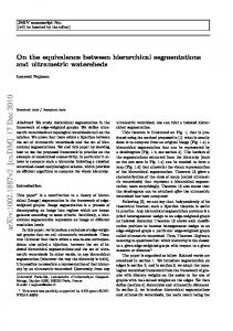
which is the only term depending on the dimensions of Ω, where a is a vector gathering the sampling-area dimensions av used in (12). Using a Monte-Carlo method and assuming a uniform angular distribution, the evolution of GΩ is plotted in Fig.1, where a line of length a (dashed line), a square of side a (dotted line) and a cube of side a (solid line) have been considered, respectively. As shown in Appendix A, the term ν4 − ν2 2 in (41) is 2 the relative-ensemble variance σr,p 2 of the mean-square pressure, defined as, [( )2 ] 2 2 (r) p (r) − µ p ω 2 ω σr,p . (43) 2 = E µ2p2 (r) ω

If no spatial averaging is performed, then GΩ (0) = 1. It follows that the variance σϵ 2 of the relative error re2 duces logically to σr,p 2 , i.e., to the relative variance of Spatial and Ensemble estimators

5

µ ˆp2ω =

1 NR

NR ∑

p2ω,i ,

(44)

0

10

−1

10 GΩ(a)

the mean-square pressure in a single point. The relativeensemble variance has been widely studied in the literature using wave theory7,23 and modal theory3–5 models and will not be analyzed in detail herein. All these models have been validated experimentally, and show that 2 the relative-ensemble variance σr,p 2 is inversely proportional to the number of overlapping modes Ms and tends to one for an ideal diffuse field, i.e, for an infinite number of plane waves. Concerning spatial averaging, the modal models of Davy4 and Weaver5 included the influence of multiple independent receivers, i.e., of independent spatial samples, in the overall relative variance. Accordingly, if we consider a single fixed source and NR independent receivers, the mean estimated value µ ˆp2ω of p2ω (r) can be deduced using an arithmetic mean, i.e., a discrete version of (7), as

−2

10

−3

10

−4

10 −1 10

0

10 a/λ

1

10

FIG. 1. Evolution of the spatial term GΩ (a) in (42). 1D, 2D and 3D sampling domains have been considered, related to a line stretch of length a (dashed line), to a square (dotted line) and a cube of side a (solid line), respectively.

i=1

hal-00614712, version 1 - 15 Aug 2011

which is the traditional mean-estimator. Using modal models4,5 , it follows that σϵ

2

1 2 = σ 2, NR r,p

(45)

where 1/NR is referred to as the convergence rate. Within the modal approach, it appears that the more (independent) receivers we take the more accurate the estimated mean value will be. This of course unrealistic because a spatial correlation exists; but as explained in section II modal models cannot include easily the effect of spatial field distribution into the moments of spatialaverage estimates. Using the plane-wave model presented herein, (41) can interestingly be restated as follows 2 σϵ 2 = G(a, N )σr,p 2,

The study of the accuracy of the spatial-average estimator consists then in analyzing the convergence rate given in (47) which can be simplified as, G(a, N ) ≃ GΩ (a) + GP W (N ),

(48)

since the term (N − 1)/N can be reasonably neglected. Accordingly, to study which of the two terms dominates in the overall estimator variance, the knowledge of 2 σr,p 2 is not needed since this latter is common. Consequently, we shall focus our analysis in the next section, on a comparison of the two terms of (48).

(46) IV. ACCURACY OF THE SPATIAL ESTIMATOR

where G(a, N ) is the convergence rate of the spatial estimator expressed as G(a, N ) =

N −1 GΩ (a) + GP W (N ), N

(47)

with GP W (N ) = 1/N . Note that on a single point, i.e., for a = 0 the convergence rate G(0, N ) = 1 as expected, independently of the number N of plane waves. It turns out that the convergence rate of the spatial estimator obtained in (47) is conditioned by two terms. The first term, as expected, is related to the influence of the sampling term GΩ (a) whose inverse corresponds to an equivalent number of independent samples. The number of plane waves has very little influence on the first term of (47). On the contrary, the second term depends only on the number of plane waves. The influence of the number of plane waves in the spatial-averaging convergence rate has never been predicted to the best of our knowledge by any study.

A. Existence of a lower bound

We are interested in comparing the two terms in (48) in order to see if the contribution of the plane waves may be significant in some cases. This is of relevant importance because the presence of the 1/N term in the variance expression acts as a lower bound in the spatialaverage estimator accuracy. Indeed, the number of plane waves is related to the room configuration, but is independent of the sampling area Ω. Consequently, if the sampling area is larger, the GΩ term will decrease, as seen in Fig. 1, but leaving the 1/N term unchanged. In practical terms, raising the sampling area will not diminish continuously the degree of uncertainty deduced from the spatial-average-estimator variance. To stress the significative risk of this limitation, we study in the next subsection practical room cases for which an assessment of the two contributing terms, i.e., of GP W and GΩ , is performed. Spatial and Ensemble estimators

6

a/λ −1 6 7 8 9 10 Small lightly damped room GPW

7

4

10

6

Convergence rate

Reverberation time [s]

−1

5 4 3 2

−2

10

10

(a)

GΩ

−3

10

200 300 400 500 600 700 800 900 Frequency [Hz] 4

−1

10

10 Frequency [Hz]

FIG. 2. Reverberation times from Ref.7. Four configurations have been considered : a large room (solid line), a large damped room (dotted line), a small room lightly damped (dashed line) and a small damped room (dashed-dotted line).

Convergence rate

3

−2

Small damped room

1 0 2 10

5

5

6

7

8

9

GPW

10

10

−3

−1

Large room −2

10

10

GΩ

(b)

Large damped room

−3

10

−2

200 300 400 500 600 700 800 900 Frequency [Hz]

10

−3

hal-00614712, version 1 - 15 Aug 2011

B. Influence of room parameters

In order to assess quantitatively the role of GP W , we consider real room configurations. We use the experimental data presented in Ref. 7 for the case of a small room (40 m3 ) and a large reverberation room (245 m3 ) with large fixed diffusers. Both rooms are essentially rectangular. For the small room, lightly damped and damped cases are considered. The corresponding Schroeder’s frequencies are 500 Hz and 330 Hz, respectively7 . For the large room very little damping and large damping cases have been considered. The corresponding Schroeder’s frequency are of 310 Hz and 200 Hz, respectively7 . The measurements of the reverberation time T60 were performed on a frequency range [100 Hz : 3.2 kHz] and is shown in Fig. 2. The configuration of a room has a direct impact on the modal topographies but also on the frequency response and consequently on the number of plane waves composing the sound field. In order to fruitfully use the experimental room parameters we need to establish a way to relate them to the number of plane waves in the following way. At a frequency f , we may consider β plane waves per resonant mode. In order to assess the number M of modes that are found within the average resonant 3dB bandwidth BM , we use the simplest form of Weyl’s approximation24 of the modal density. The number of plane waves involved in the sound field can then be approximated as N = β · M = β n(f )BM ≃ β

4πV f 2 BM , c3

(49)

where n(f ) is the modal density (in modes per Hertz), V is the volume of the room and c the sound speed. Recalling that the reverberation time T60 is related to the average bandwidth of a mode BM , such as BM = 6.91/π · T60 yields the following expression of the plane-

FIG. 3. Comparison of the lower bound GP W as a function of frequency (lower x -axis) (with ten plane waves per mode) with the 2D-square spatial term GΩ as a function of a/λ (upper x -axis) for (a) the small room configurations and (b) the large room configurations of Ref. 7. A value of 3.3 m was considered for the parameter a.

wave term in (48) GP W =

c3 T60 , 27.64 β V f 2

(50)

providing a relation allowing to assess the lower-bound term using the room reverberation time T60 and the room volume V . For the four room configurations, Fig.3 shows the evolution of GP W as a function of frequency (lower x -axis), and the evolution of the spatial GΩ term as a function of a/λ in the 2D case for 3 < a/λ < 10 (upper x -axis) where a value of 3.3 meters has been assumed for the parameter a. As already said, the number of plane waves per mode is hard to estimate. The rooms being essentially rectangular we can expect approximately eight plane waves per mode. In order to consider an upper bound we use a value of ten plane waves per mode. We stress that this value being used for all the modes on average, the GP W term may not be regarded as overvalued. For the case of the small room Fig.3a shows that the plane-wave term dominates even for frequencies above Schroeder’s frequency, whereas for the large room cases described in Fig.3b, the two terms are of the same order of magnitude. These results can be regarded as a further proof to the well-known fact that the acoustics of small rooms are in a way more complicated than those of large ones. In the present case, it is an illustration that, at a given frequency, the smaller the room the worse the accuracy of the spatial estimate will be; not only because of the relative-ensemble variance as commonly known, but Spatial and Ensemble estimators

7

10

0

T60=6 sec@1kHz

Convergence Rate

α=0.1

10

α=1

10

10

10

−2

−3

T60=1 sec@100Hz −4

10

hal-00614712, version 1 - 15 Aug 2011

T60=3 sec@1kHz

−1

0

1

10

2

10

Vλ

10

3

4

10

5

10

FIG. 4. GP W (bold line) and GΩ (solid line with circles) as a function of the acoustical volume Vλ of a room. GΩ is related to the 2D-section of the sampling volume for which two cases are considered : the sampling volume fits the entire room volume (α = 1) and only 10% of the room volume is used in the second case (α = 0.1). For GP W , frequencies below and above Schroeder’s frequencies have been chosen (100Hz and 1kHz, respectively) and three values of reverberation times given in Fig. 2 were used, namely the minimum value of 1 s, the maximum value of about 6 s and an in-between value of 3 s.

also due to the spatial-averaging effect assessed herein. In both cases of Fig. 3, the finite number of plane waves has an influence on the overall convergence rate not only for frequencies near Schroeder’s limit, as intuitively expectable, but in fact for a frequency range whose upper limit would be approximately ten times Schroeder’s frequency. At this stage a comparison between GP W and GΩ (a) has not been performed on the basis of a common parameter. To this end, we consider that the 3D-sampling zone, referred to as Ω3D , is a portion α of the room volume V , such as Ω3D = αV . In order to include the influence of the frequency (or equivalently the wavelength λ) at which the measurement is performed, we introduce the acoustical sampling volume defined as Ω3D = Ω3D /λ3 . λ Equivalently, we define the acoustical volume of the room defined as Vλ = V /λ3 , yielding GP W =

T60 f . 27.64 β Vλ

(51)

The computation of GΩ requires the dimensions of the rooms. These latter being not known, we consider the following geometrical ratios 3 : 4 : 5, related to the width a1 , the height a2 and the length a3 of the sampling volume, respectively. These ratios account for the absence in practice of degenerate eigenfrequencies. For the sake of plotting clarity, we restrict the analysis to the a2 a3 section, referred to as Ω2D , of the sampling volume Ω3D . To compute the resulting GΩ term, two cases of Ω3D are considered : the case for which the sampling volume fits the total room volume, i.e., for α = 1, and the case for which the sampling volume repre-

sents 10% of the room volume, i.e., for α = 0.1. Accordingly, Fig.4 shows the resulting 2D-GΩ term for α = 1 and α = 0.1, and the plane-wave term. For this latter, frequencies below and above Schroeder’s frequency were considered, 100 Hz and 1 kHz, respectively, and three values of reverberation times were chosen on the basis of the experimental data provided by Fig. 2. The selected values correspond to the minimum of 1 s, to the maximum of about 6 s and to an in-between value of 3 s well suited to the large damped room and small lightly damped room cases. We can see in Fig. 4 that at a fixed frequency (1kHz in the present case), the decrease of the reverberation time induces a lower convergence rate as stated by (51). If the frequency f varies, so does the acoustical volume since this latter is a function proportional to the cube of f . If we refer to the large and small rooms cases, taken at 1 kHz, respective acoustical volumes of 6000 and 991 are found. Using Fig. 4 for α = 0.1, we find that GP W = GΩ = 10−2 for the small room; for the large room, GP W = 2 10−3 and GΩ = 3.5 10−3 . This illustrates the influence of the plane-wave term, since it contributes, for the small room case, to 50% of the overall convergence rate.

TABLE I. For sampling volumes corresponding to 10% (α = 0.1) and 100% (α = 1) of the small- and large-room volumes, respectively, relative margin of errors mr,ϵ and the corresponding 2D sampling areas Ω2D are reported. The number Neq of equivalent independent spatial samples is also reported for α = 0.1, assumed as a more realistic case. Configuration α=1 small room α = 0.1 α=1 large room α = 0.1

mr,ϵ 20% 28% 10% 15%

Ω2D Neq 31m2 6.8m2 100 105m2 22m2 250

In practice, the spatial-average estimate expressed in (7) can be regarded as a random Gaussian variable whose relative standard deviation σϵ conditions the confidence interval, i.e., the accuracy of the estimator. We define the margin of error mϵ value as the half-width of the confidence interval. If we consider that 95% of the cases fall into this latter, the margin of error is approximately mϵ = 2σϵ . Our concern dealing with the comparison of the two terms of (48), the estimator efficiency can be described by 2 the √ following relative margin of error mr,ϵ = mϵ /σr,p = 2 GΩ + GP W , plotted in Fig. 5 as a function of the acoustical volume of the room, for the 1D (triangles), 2D (circles) and 3D (squares) cases. For the plane-wave term a reverberation time of 3 s at 1 kHz has been used. We consider the cases for α = 1 (solid line) and α = 0.1 (dashed line) in order to assess the influence of the sampling area on the uncertainty range related to the spatial estimator efficiency. Spatial and Ensemble estimators

8

esis. To the best of our knowledge, no other studies have been presented in a more general case. Accordingly, it is interesting to analyze how the general expression, given in (46), becomes in the particular case of an ideal diffuse field.

2

Margin of error mr,ε [%]

10

1

10

C. The ideal diffuse field case 1. Relative variance expression

0

10 2 10

3

10

4

Vλ

10

5

10

hal-00614712, version 1 - 15 Aug 2011

FIG. 5. The relative margin of error related to (48) for a 95% confidence interval and a reverberation time of about 3 s at 1 kHz. Sampling volumes in 1D (triangles), 2D (circles) and 3D (squares) are considered. The case for which the sampling volume Ω fits the entire room volume (α=1) is plotted in solid line - the case for which the sampling volume is 10% of the room volume is plotted in dashed line.

If we refer to the practical cases described previously for which GP W = GΩ = 10−2 for the small room and GP W = 2 10−3 and GΩ = 3.5 10−3 for the large room, we find the respective relative margins of error of 20% and 10% for α = 1, and 28% and 15% for α = 0.1. Regarding the GΩ term as an inverse number Neq of equivalent independent discrete spatial samples, 100 and 250 equivalent samples are found for the small and large room, respectively, for α = 0.1. All these values are summed up in Tab. I where the equivalent sampling 2Dareas Ω2D have also been reported providing the order of magnitude of the surface related to the relative margins of error previously mentioned. Interestingly, if the α = 0.1 case of the spatial estimator were replaced by an ensemble estimator (using a rotating vane or moving the source and receiver positions as in Ref.7) based on Ns independent samples, we would need, on the basis of the same margins of error, i.e., 28% and 15%, 51 and 177 samples for the small and large room, respectively. For the small room case, to compensate the plane-wave term GP W , a spatial-averaging process needs twice more independent samples than an ensemble estimator. It is worth stressing that in the case of an ensemble estimator, each realization corresponds to the case of G(0, N ) = 1, i.e., the number of plane waves has no influence. The method presented herein can be then extended in a general way to any configuration. It provides a practical theoretical tool for predictions and estimation procedures applied to the mean-square pressure in room acoustics. In the general model derived in section III, we did not make any assumption on the degree of diffusion of the field unlike the works dedicated to spatial averaging in the litterature13,15–18 . Indeed, these latter have been carried out within the frame of the ideal diffuse field hypoth-

In the case of an ideal diffuse field, i.e., for an infinite number of plane waves, using (47), we can show that the convergence rate G(a, N ) reduces to GΩ (a). The relative-error variance of the spatial estimator given in (46) can then be expressed as 2 lim σϵ 2 = GΩ (a) σr,p 2.

N →∞

(52)

The relative-ensemble variance of the mean square pres2 sure σr,p 2 can be analyzed in a straightforward way. Indeed, the complex plane-waves weights {w} in the new basis result from an infinite sum of the {γ} random variables. Accordingly, using the central limit theorem, we can state that the real and imaginary parts of the set {w} follow a normal distribution. Consequently, the elements |wi |2 follow a chi-square distribution with two degrees of freedom whose moments are such that ν4 E[|wi |4 ] = 2 = 2. E[|wi |2 ]2 ν2

(53)

Hence, recalling that E[|wi |2 ] = 1, the relative variance 2 σr,p 2 reduces to unity as commonly accepted for the ideal diffuse field case. We can then express (52) in the following simpler form lim σϵ 2 = GΩ (a),

N →∞

(54)

which is the expression given by Schroeder13 . In Schroeder’s work13 a Gaussian assumption is made on the {γ} set distribution. Note that, in the model derived in section III such assumption is not necessary to recover the expression of the error variance in the case of an ideal diffuse field.

2. Estimators equivalence

In order to analyze if a spatial- and ensemble-average estimators are equivalent, one needs to compare their convergence rates. To this end, we introduce the ensemble-meanestimated value of the mean-square pressure µp2ω defined as, µp2ω =

Mr 1 ∑ p2 , Mr i=1 ω,i

(55)

where p2ω,i is the mean-square pressure corresponding to the i-th realization of the ensemble statistics and Mr is Spatial and Ensemble estimators

9

hal-00614712, version 1 - 15 Aug 2011

valid for a/λ > 2. These expressions, derived for the first time for the 2D and 3D cases to the best of our knowledge, allow to see the impact of the dimensionality of Ω on GΩ slopes. The difference of slopes, linked to the difference of exponent power value in the asymptotic expressions of GΩ , is induced by the spatial correlation of the field in the room. The correlation effects on the spatial variance have already been studied in the cases of a line, a circle and a disk sampling areas15–17 . For the mean-square pressure, the spatial autocorrelation function R(k0 ∆r) was shown to be17,25 , ( )2 sin(k0 ∆r) R(k0 ∆r) = , (57) k0 ∆r where ∆r is the distance between two points. Using (57), a zero correlation is found for distances of λ/2, or entire multiples. On the basis of this property, the ensuing idea of using a discrete, rather than a continuous, spatial-average estimator has been studied by Waterhouse18 who was interested in studying the different possible arrangements in 1D, 2D and 3D to have uncorrelated discrete samples. It can be shown that the 1D equivalent discrete averaging estimator, i.e., sampling along a line on positions apart from λ/2 (or multiples), is the only case for which uncorrelated samples can be obtained. Indeed, in the 2D and 3D cases no geometrical configuration can provide a zero correlation between

−1

10 Estimator relative variance

the number of independent realizations. A realization can either be a position of a rotating vane or a pair of source/receiver positions. If the total number Mr of realizations are independent, µp2ω is a random variable whose centered and normalized form, as done in (13), follows a normal distribution of zero mean and of vari2 ance σr,p 2 /Mr . The spatial-average (centered and normalized) estimate ϵ follows also a normal distribution with a zero mean. However, the variance and/or convergence rate is not identical in all the spatial-sampling configurations as shown in Fig. 1. Indeed, we observe different slopes preventing a general equivalence principle between spatialand ensemble-average estimates as the confidence interval is not identical. Accordingly, the claim in Ref.17 that the spatial-average estimator provides the ”true estimate” is not correct in a strict sense although the 1D/2D/3Dspatial-variances GΩ tend asymptotically to zero. In order to carry on a more accurate comparison of the convergence rates of µ ˆp2ω and µp2ω , we focus on the different slopes of GΩ for the 1D, 2D and 3D cases which turn to be 0.5, 0.4 and 0.26 per octave, respectively. For the 1D case, the slope is in accordance with the asymptotic expansion of the expression of Ref.13. For the 2D-square and 3D-cube cases no analytical expressions being available, we have estimated the following asymptotic expressions   0.5/(a/λ) in the 1D case  GΩ (a) ≃ 0.2133/(a/λ)1.8 in the 2D case (56)   0.0740(a/λ)−2 in the 3D case

−2

10

−3

10

−4

10

1

10

2

3

10 10 Number of samples

4

10

FIG. 6. Variance of the spatial-average estimator in the 1D (triangles), 2D (circles) and 3D (squares) cases with respect to the ensemble-mean estimator (solid line with no markers), as a function of the discrete number of samples.

each pair of points. Consequently, in the 1D case, doubling the number of (independent) samples, i.e. doubling a/λ, will reduce the estimator variance σϵ2 of a factor 2, confirming the slope obtained in the 1D case in Fig.1. To compare GΩ with the convergence rate 1/Mr of the ensemble estimator, we need to use a discrete spatialaverage estimator in order to have the number samples as a common parameter. It has been shown18 that the relative-error variance of the discrete spatial-average estimator can be fairly approximated by GΩ , as long as the geometric parameter a is greater than 3/2 λ. Accordingly, assuming a sufficient number of samples allows using (56) to describe properly the asymptotic convergence rate of the discrete spatial-average estimator. In order to compare the convergence rates of the two estimators, we need to introduce a number of spatial samples whose arrangement will impact inevitably on the accuracy of the spatial-average estimate. We choose a regular arrangement of the samples separated by a distance λ/2. This arrangement allows, on the one hand, to have samples easily placed and on the other hand, to have a zero-correlation in many cases. If Ns is the number of samples in the 1D case ensuing from the regular arrangement, Ns2 and Ns3 will be the samples obtained in the 2D-square and 3D-cube cases, respectively. Moreover, if a length a is assumed for the 1D case, the integer part of 1 + a/(λ/2) correspond to the number of samples. Equivalently, for a sufficient value of a, we have approximately 2a/λ samples along a line or along the side of a square and a cube of length a. Consequently, using the asymptotic approximations of GΩ we can compute the following asymptotic convergence rates    Ns−1 in the 1D case GΩ (Ns ) ∝ (58) Ns−0.9 in the 2D case   N −0.666 in the 3D case s Spatial and Ensemble estimators

10

Using the results of GΩ shown in Fig.1, we plot in Fig.6 the variance of the relative error of both estimators as a function of the number of samples. The 1D case and the ensemble estimator being based on independent samples, they converge with the same rate. Whereas, the 2D and 3D cases are affected by spatial correlation. Consequently, their convergence rates are lower. Accordingly, for the scenarios where the ideal diffuse field model can be assumed as reliable, the ofteninvoked equivalence assumption between spatial-average (in the 2D and 3D cases) and ensemble-average estimators does not hold.

2 2 σr,p 2 = ν4 − ν2 .

1

2

3

V. CONCLUSION

hal-00614712, version 1 - 15 Aug 2011

Recalling that ν22 = 1, the final variance is obtained comˆ set. However, puting the conditional average on the {k} ˆ set, finally yielding ν4 is independent of the {k}

The present study showed that the spatial- and ensemble-average estimators cannot be regarded as equivalent, since their convergence rates differ. The results were obtained using a wave-theory approach based on a finite number of plane waves; the plane-wave model is equivalent to a modal expansion, while allowing to explicitly express the spatial dependence of the sound-field distribution, well-suited to the study of the spatial estimator. For an infinite number of plane waves the spatialaveraging estimates coincide with the results presented forty years ago using an ideal-diffuse field model. In the general case, the present work points out theoretically that the number of plane waves induce a limitation of the spatial-estimator accuracy, emphasizing the uselessness of over-sampling. This effect has never been predicted to the best of our knowledge. On the basis of practical cases, the results show that this effect impacts the convergence rate for frequencies about ten time Schroeder’s frequency. Although the model is physically justified and theoretically reliable, it would be interesting to establish this limitation on the basis of experimental measurements. These studies would provide an experimental evidence of the maximum accuracy that can be expected.

4

5

6

7

8

9

10

11

12

13

14

15

APPENDIX A: IDENTIFICATION OF THE VARIANCE 16

2 σr,p 2

In order to identify the relative-ensemble variance of the mean-square pressure defined as, [( )2 ] [ ] p2ω (r) − µp2ω (r) 2 = E ϵ2 , (A1) σr,p2 = E µp2ω (r) we must consider the error expression in (13) in a single point. The matrix P is then made of ones. Consequently, the matrix being of unitary rank, we have only a single non-zero eigenvalue λ1 such as, λ1 = N.

17

18

19

20

21

(A2)

Accordingly, (32) can be expressed with the following simpler form, [ ] Ew ϵ2 = ν4 − 1. (A3)

22

23

(A4)

M. Schroeder, “Statistical parameters of the frequency response curves of large rooms”, J. Audio Eng. Soc 35, 299– 305 (1987). M. Schroeder and K. Kuttruff, “On frequency response curves in rooms. comparison of experimental, theoretical, and monte carlo results for the average frequency spacing between maxima”, J. Acoust. Soc. America 34, 76 (1962). R. Lyon, “Statistical analysis of power injection and response in structures and rooms”, J. Acoust. Soc. America 45, 545 (1969). J. Davy, “The relative variance of the transmission function of a reverberation room”, Journal of Sound and Vibration 77, 455–479 (1981). R. Weaver, “On the ensemble variance of reverberation room transmission functions, the effect of spectral rigidity”, Journal of Sound and Vibration 130, 487–491 (1989). R. Waterhouse, “Statistical properties of reverberant soundfields”, J. Acoust. Soc. America 35, 1894 (1963). F. Jacobsen and A. Molares, “The ensemble variance of pure-tone measurements in reverberation rooms”, J. Acoust. Soc. America 127, 233 (2010). C. Balachandran, “Random sound field in reverberation chambers”, J. Acoust. Soc. America 31, 1319 (1959). F. Jacobsen and T. Roisin, “The coherence of reverberant sound fields”, J. Acoust. Soc. America 108, 204 (2000). H. Kuttruff, Room acoustics, chapter 3, 86–88 and 76, 5th edition (Spon Press, Oxon) (2009). W. Joyce, “Sabine’s reverberation time and ergodic auditoriums”, J. Acoust. Soc. America 58, 643 (1975). M. Witting, Modelling of diffuse sound field excitations and dynamic response analysis of leightweight structures, chapter 2, 10 (Herbert Utz Verlag, M¨ unchen) (1999). M. Schroeder, “Spatial averaging in a diffuse sound field and the equivalent number of independent measurements”, J. Acoust. Soc. America 46, 534 (1969). M. Schroeder, “Effect of frequency and space averaging on the transmission responses of multimode media”, J. Acoust. Soc. America 46, 277 (1969). D. Lubman, “Spatial averaging in a diffuse sound field”, J. Acoust. Soc. America 46, 532 (1969). D. Lubman, “Spatial averaging in sound-power measurements”, J. Acoust. Soc. America 45, 337 (1969). D. Lubman, R. Waterhouse, and C. Chien, “Effectiveness of continuous spatial averaging in a diffuse sound field”, J. Acoust. Soc. America 53, 650 (1973). R. Waterhouse and D. Lubman, “Discrete versus continuous space averaging in a reverberant sound field”, J. Acoust. Soc. America 48, 1 (1970). P. M. Morse and K. U. Ingard, Theoretical Acoustics, chapter 9, 556–558 (McGraw-Hill, Inc., New York) (1968). R. Lyon, “Needed: a new definition of diffusion”, J. Acoust. Soc. America 56, 1300 (1974). P. Chinnery and V. Humphrey, “Experimental visualization of acoustic resonances within a stadium-shaped cavity”, Physical Review E 53, 272 (1996). A. Papoulis, Probability, random variables, and stochastic processes, chapter 9, 245–247, 2nd edition (McGraw-Hill, Inc., New York) (1984). F. Jacobsen and A. Molares, “Sound power emitted by a

Spatial and Ensemble estimators

11

25

body theory))”, Mathematische Annalen 71, 441–479 (1912). W. Chu, “Note on the independent sampling of meansquare pressure in reverberant sound fields”, J. Acoust. Soc. America 72, 196–199 (1982).

hal-00614712, version 1 - 15 Aug 2011

24

pure-tone source in a reverberation room”, J. Acoust. Soc. America 126, 676 (2009). H. Weyl, “Das asymptotische Verteilungsgesetz der Eigenwerte linearer partieller Differentialgleichungen (mit einer Anwendung auf die Theorie der Hohlraumstrahlung)(Asymptotic distribution of the partial differential equations eigenvalues (with an application to black

Spatial and Ensemble estimators

12