that exponential smoothing and 'naive' models, previously thought to be 'robust' performers, forecast poorly for the particular set of time series under analysis, ...
International North-Holland
Journal
of Forecasting
81
8 (1992) 81-98
The evaluation of extrapolative forecasting methods Robert
Fildes
Lancaster University, Lancaster, UK
Abstract: Extrapolative forecasting methods are widely used in production and inventory decisions. Typically many hundreds of series are forecast and the cost-effectiveness of the decisions depends on the accuracy of the forecasting method(s) used. This paper examines how a forecasting method should be chosen based on analyzing alternative loss functions. It is argued that a population of time series must be evaluated by time period and by series. Of the alternative loss functions considered, only the geometric root mean squared error is well-behaved and has a straightforward interpretation. The paper concludes that exponential smoothing and ‘naive’ models, previously thought to be ‘robust’ performers, forecast poorly for the particular set of time series under analysis, whatever error measure is used. As a consequence, forecasters should carry out a detailed evaluation of the data series, as described in the paper, rather than relying on a priori analysis developed from earlier forecasting competitions. Keywords: Evaluation - time series methods, Evaluation - methodology, Comparative series, Robust estimation, Outliers - effect of, Loss functions - evaluation, Ex ante.
The statistical evaluation of the forecasting performance of extrapolative time series methods is important for any applied forecaster trying to decide which method to use. In inventory/production control applications the researcher will typically need to consider a method’s performance on a (potentially) large number of series. This paper identifies guidelines for carrying out such evaluations. The first section of the paper describes the various loss functions that are used in the context of inventory control. They are evaluated theoretically by reference to certain simple error models. The second section details the data used and the forecasting methods that have been applied in an attempt to understand the behaviour of these loss functions. These performance statistics are analysed in section three in the context of a forecasting competition based Correspondence to: R. Fildes, Department of Operational Research and Operations Management, Management School, Lancaster University, Lancaster LA1 4YX, UK. 016Y-2070/92/$05.00
0 1992 - Elsevier
Science
Publishers
methods
- time
on the analysis of 263 series. The final section concludes by comparing the results of this forecasting competition with those of earlier studies, in particular, Makridakis et al. (1982). The dangers of mis-interpreting forecast error statistics through the use of inadequate test statistics are demonstrated and procedures for avoiding their worst effects are suggested.
1. Loss functions
in forecast error analysis
An extrapolative (time series) model of a particular time series uses only the history of the s:ries in forecasting its future values. Formally: Y,(k) =f(Y,, YT_ ,,... YT_-p...), where YT(kl is the k step-ahead forecast of YTtk made at time T based on data available to T. Statisticians have developed criteria for selecting the lag length p and functional form so that Y,(k) is an ‘optimal’ predictor, evaluated against some preselected loss function. The principal statistical rules that are
B.V. All rights reserved
applied rely on some modification of the estimated standard deviation of the forecast error by factors which depend on the number of parameters and number of observations, eg. Akaike’s Information Criterion (AIC). [For a survey see de Gooijer et al. (198511. All these measures are based on parameters (typically the error variance) estimated within sample. However, both simulation studies and empirical studies such as Newbold and Granger’s (1974) showed that these identification procedures were inadequate. Knowledge that both formal and informal methods of identification were unsatisfactory led inexorably to the conclusion that statistics of fit alone could not be used as a basis for model choice. Instead, researchers resorted to using a combination of within-sample error statistics to limit the range of models to be considered, and outside sample error statistics to test the models. f. 1. Outside sample error ~rl~a~ur~s A wide range of error measures based o? the k-step ahead forecast error e,(k) = Yr+k - Y,(k) has been used in the attempt to provide evidence on forecast performance. When attempting to compare forecasting pe~ormance over a number of series such as is required in the various forecasting competitions, eg. Makridakis et al. (19821, a large number of forecast errors must be summarized as is illustrated diagrammatically in Exhibit 1. The error, ejj, is the error made in forecasting the T,, +j th data point of series i, lead time
Exhibit 1 The forecast error matrix (Forecast lead time, Lf.
and corres~nding
summa~
error
being assumed fixed and where T,, is the time origin of the data used for the evaluation. For any given time period, T,, +j(j > L - I), there are N L-step ahead forecast errors which can be aggregated to form two (or more> error measures, the ‘Time Squared Error’ (TSE) based on a square error measure calculated 6y time period across series and ‘Time AbsoIute Percentage Error’ (TAPE) based on absolute percentage error. [Other alternatives could also be included but measures based on either squared error or absolute percentage error are most commonly used, Carbone and Armstrong (1982)]. For any given series, there are ?‘- L + 1 L-step ahead errors which can be aggregated across time to form summary measures ‘Series Squared Error’ (SSE) and ‘Series Absolute Percentage Error’ (SAPE). A similar data matrix can be generated for each set of lead time forecasts. The various competitions incIuding the Makridakis competition (M-Competition} only included error statistics aggregated across series for one particular time origin. Such error statistics have been analysed by Makridakis and Winkler (1989) who concluded the outside sample errors in the M-Competition bear iittle reIationship to the within-sample errors. Jenkins (1982) makes the criticism that with only one time origin used as a basis for all forecasts the possibility exists that the arbitrary choice of time origin might unduly have affected the results. Of course, if the data series were stationary, this would not be a matter of serious concern. Without the stationarity assumption however, many of the conclusions that have
measures.
Series Time
T,,
+
T
Summary Summary measures series
by
N
Summary measures time period
1
2
_
_
_
elL
e2/.
TSE.,
e,r
e27.
eN7.
SSE, SAPE,
SSE, SAPE,
SSE, SAPE,
by
TAPE.
L
TAPE ,TSE 7 Overall summary measures SSE... TSE...
SAPE... TAPE..
83
R. Fiides / Extrapolatiic*eforecasting methods
been drawn from the various forecasting competitions might be undermined by nonstationary sampling variability across time ‘. 1.2. Models of forecast error in inventory control Forecasting comparisons of the type we describe are necessary in production and inventory applications. A single general loss function can seldom capture the complexities of how forecasting models are used. For example, Price and Sharp (1986) show how standard statistical accuracy measures inadequately capture the specific loss function appropriate to investment in electricity supply. Nevertheless, in inventory control applications where in practice simple inventory control schemes are used, one important measure of loss is the safety stock investment (although it neglects stock out costs), KsC,cj,, where K is the safety factor, C, is the unit value of the ith product and ci is the forecast error standard deviation over the replenishment Iead time. However forecasting researchers have, perforce, adopted a wide range of general loss functions typically based on squared or percentage error measures, hoping the practitioner trying to use the results would find a loss function that approximately matched the problem in hand. The (fixed lead time) errors (and associated loss functions such as SSE) for a particular series are, in theory, well-behaved with each forming their own empirical distribution which can be compared with an appropriate theoretical distribution and summarised by a,, Mean Square Error and MAPE etc. However the error distributions and the error statistics calculated across series for a given time period are less easily interpreted unless the data series can be thought of as a sample from a well-defined population of series. Without that necessary homogeneity, the MSE is uninterpretable as discussed by Gardner (1983), Newbold (1983) and Fildes (1983); the MSE statistics and the mean standard deviation are scale dependent and a method can be ranked first on MSE just because it scored particularly well on perhaps the one series with typical errors ’ Jenkins
also criticizes the practice statistics across lead time, a criticism this paper all analyses are carried pre-specified lead times.
of aggregating error with which I agree. In out for a number of
significantly larger than the remaining series [Chatfield, (1988)]. Scale dependence is a severe weakness in an error measure applied to business problems in that the unit of measurement in which a series is recorded is often arbitrary. Similar, though less significant criticisms, can be levelled at the MAPE as Gardner (1983) points out and these again arise because the sampling distribution for MAPE measured across series is often badly positively skewed. MAPE also suffers by being sensitive to location in that a change of origin in the data affects the MAPE. However the origin in business series is typically well-defined. Because of its widespread use we consider MAPE in our subsequent analysis. The problem posed by scale dependence can be understood by considering the following model. Suppose the squared errors are of the form:
where eirM (Ll is the L-step ahead error made in forecasting period t + L for series i using method M, and where ’ * ’ could represent either an additive or multiplicative relationship. The I’~,, are assumed positive and further that they subsume any serial relationship in the errors and fei,,JL)} are assumed to be stationary. The t~;~can be thought of as errors due to the particular time period affecting all methods equally while the {e,,,,,,(L)} are the method specific errors. Dropping the lead time for convenience, such a model effectively represents the case where the data (and errors> are contaminated by occasional outliers. When such a model holds, a ‘Series Sauared Error’ measure, SS&,,
such as
~~~~i~) could potentialiy be dominated by the (z!~,},and accordingly, comparison of two forecasting methods, M, and M,, would also be unduly affected. The inventory control loss function should not depend on {tit}. As argued earlier they are best seen as occasional outliers and therefore any automatic forecasting system should not be geared to respond to such extremes. Rather they shouid be dealt with by an exception monitoring scheme. Particularly important for the purposes of this paper, the choice of forecasting method to employ should not be dependent on such extremes except in so far as one method extracts whatever
R. Fildes / Extrapo1atiL.eforecasting methods
84
information there may be in an outlier better than another. The contamination of SMSE by series can be overcome by adopting the Geometric Root MSE’. The Geometric Root Mean Square Error by series (SGRIMSE,,) for a particular series is calculated as shown below: jne:,+ t
where n = T - L + 1 and is the number of effective data points. Using the equation e” GRhk~“?k!~~ &(L) * Ul,(r+LY the relative . time) of method 1 compared to method 2 (ijlWV~4~W)~~
= (~41cl,/~4#4)k E,:I(L)
= 4f
42(L)
; i
which is independent of {L’~~} if they are assumed to have a multiplicative effect. Both absolute and relative error measures have the advantage over the conventional RMSE in that they are scale independent. Interpretation is straightforward: a method with GRMSE 10% greater than an alternative has on average a 10% larger absolute error per series. In addition, if a forecasting method has absolute error on one series 10% higher than the alternative and on another 10% lower, the GRMSEs are equal when averaged across these two series. Eg. Suppose for series 1, method 1 has SE, of 110 compared to method 2 at 100 while on series 2, method 1 has SE, of 1000 compared to method 2’s 1100, then: Relative GRMSE = ((llO/lOO) = 1 while the Relative Arithmetic
*(1000/1100))1’2
RMSE
arises solely because of its better performance on series 2, the series with the larger observations. Now if Geometric Root Mean Squared Error, GRMSE, by series (SGRMSE) can be modelled as log normal, then Relative SGRMSE, is also log normal 3. Similarly GRMSE by time period may be assumed log normal and the summary measures of the distributions by series and by time period have the important property that they are equal, i.e. Relative SGRMSE. ,= Relative TGRMSE.. = Relative GRMSE,
where the double dot notation implies the statistics have been calculated over both the available time periods and the N data series. In summary, the following assumptions have been made which, if supported by the data, argue strongly in favour of including Relative GRMSE as one of the range of descriptive statistics useful in interpreting competitions. (1) Relative Geometric Root Mean Squared Error by Series (SGRMSE) and Relative GRMSE by Time Period (TGRMSE) can be represented by the log normal distribution for all lead times. (2) The one-step ahead relative squared errors are independent, while the relationship in the absolute squared errors may well reflect serial correlation in the {cil}. (3) The raw squared error distributions, both by series and by time period contain multiplicative outliers. As a consequence, the relative error distributions will be better behaved and more readily interpretable than the absolute error distributions. Thompson (1990) has proposed a variant of the relative GRMSE for similar reasons to those just proposed, the log relative MSE. Other error measures such as the MAPE, Median APE etc and their relative variants will depend to a greater or lesser extent on the IL:~,}~.Equally important,
= {(Ho* + 1000~)/(100~ + 1100~)}‘~2 = 0.911. The method
Relative Arithmetic MSE suggests that 2 is better than method 1 but this result
’ The measure
has long been known for averaging ages and was first used in forecasting com~risons bold and &anger (1974).
percentby New-
Strictly, for a linear combination of two normal variables to be necessarily normal, the two must be multivariate normal. A referee notes that the mean squared percentage error is often used in econometric work. While being scale independent it is likely to suffer from being unduly affected by outliers; it is also location dependent and is therefore likely to be skewed.
R. Fildes / Extrapolative forecasting methods
all measures based on APE suffer from the lack of equivalence across series and across time.
2. Forecasting
85
methods
and data
2.1. The data 1.3. An ideal error measure? Where there is no appropriate problem specific error dependent loss function, any error measure should ideally offer as full a summary of the corresponding error distribution as is possible. Therefore the summary error measures such as SSE,, SAPE,, TSE,, TAPE, (defined in Exhibit 1) should be efficient estimators of some parameter of interest from the corresponding underlying error measure distribution. The distribution itself should be well behaved in that there should be few outliers and it should be stationary over time. The error measure should not be scale dependent. Without these modest properties the analyst could find him/herself, for example, examining the mean of a highly skewed distribution with outliers, forgetting that this offers little if any information that is useful about the distribution. Thus, the choice of error measures to summarize the error distribution should not merely be a question of personal preference, as one commentator on an earlier draft of this paper noted, but rather, the forecaster must establish appropriate scaling and distributional assumptions for the data under analysis. As a consequence of these constraints there are only a limited number of valid error measures that can reasonably be adopted. The aim of this paper is: (1) to examine the empirical statistical properties of certain error measures in order to illustrate various patterns in their behaviour and to suggest reasons why some measures are likely to be better behaved than others; (2) to show how the sampling variability of error measures can lead to mis-interpreting the results from forecasting competitions. The results of the case study that lies at the heart of this analysis also underline the data specific nature of the accuracy rankings of alternative forecasting methods in any forecasting competition. Methods that perfomed well in the M-Competition, on these data series, turn out to be substantially less accurate than methods designed to capture the particular characteristics of the data being analysed.
The data used for this experiment on the evaluation of forecasting methods were collected from a telephone operating company and record the number of circuits in service by locality, available for special telecommunications services such as digital transmission. Forecasts for these series are required monthly in the company for at least 12 months ahead and form the basis for its investment in circuits and exchanges. The data are from a single US state collected over the same time scale and therefore form a homogenous population of time series. Grambsch and Stahel (1990) discuss its characteristics in more detail. They are non-seasonal with trend. An illustrative graph of two the series is shown in Exhibit 2. 2.2. Forecasting methods Comparisons of forecasting performance have become increasingly popular as the review by Armstrong (1984) makes clear. The major study was carried out by Makridakis and his colleagues (1982) which attempted to synthesise the earlier research, and overcome the criticisms that had been levelled at these so-called forecasting competitions. The M-Competition and the various authors who analysed its results have, over the years since publication, moved towards a consensus on which methods performed well overall. ’ See for example, Fildes and Lusk (198.5) and Makridakis (1983). The methods which performed particularly well in the analysis of the M-Competition data were: (0) exponential smoothing, (1) Holt’s method of exponential smoothing which includes trend, (2) Gardner-McKenzie’s damped trend (1986). Preliminary analysis of the data used in this study, [confirmed by the analysis performed by Grambsch and Stahel (1990)] show most of the series to contain strong negative trends with only six exceptions. This suggested that simple expo-
5 Since the data under analysis here are non-seasonal, eration
is limited
to non-seasonal
forecasting
models.
consid-
where the error is assumed to follow a stable distribution with shape parameter ar < 2. A stable distribution has ‘fat tails’ and is therefore suitable for modelling data where extreme values may be regularly observed. A robust estimator of the constant trend parameter y, based on observations up to t is as follows:
where m, is the median of the first differences {Aj = Y, - Y,_,) for j = 1 up to time t, and s, = median of the absolute deviations (I dj - m, I), j=l . . . t, and $(x) is a weighting function which damps out extreme deviations from the median. The 4 function used is as follows:
Time
Exhibit 2. Time series
plot of two series.
nential smoothing would perform badly and prelimina~ analysis confirmed this. It has therefore been excluded from subsequent analysis. Formulae for the above models are given in Gardner (1985). The optimal smoothing parameters have been calculated based on the first 23 data points leaving 48 data points for the subsequent analysis of ex ante errors. InitiaIisation has been carried out on the first 8 data points using Gardner’s approach and a sequential grid search adopted to establish optimal parameters. The Gardner-McKenzie formulae were used although the grid search included all three parameters for the Damped Trend model in contrast to Gardner’s AUTOcAST II. The results obtained on a sample of approximately 20 series were broadly comparable to those produced by AUTOcAST. The data described above had already been analysed by the company from which they derive and two methods found to perform well as described by Grambsch and Stahel(l990). They are: (3) Robust (4) Filter. These
Trend, methods
are briefly
described
below.
Robust Trend estimation is based on ideas of robust regression with the formulae shown below derived from the assumption that Y, is best modelled as a random walk with constant trend: dY,=y+e,,
$(x)
=2x/3
for
$(x)
= isgn(x)
IX/ < 1.5: for
~(~)=(6-~sgn(~~))/3 tcf( x) = 0 where
1.5