Al-Yasi et .al
Iraqi Journal of Science. Vol 54.No.2.2013.Pp 358-367
The Exploitation of Dar-Zarrouk Parameters to Differentiate Between Fresh And Saline Groundwater Aquifers of Sinjar Plain Area. Ameen I. Al-Yasi , Nawal A. Alridha and Wadhah M. Shakir* Department of Geology , College of Science ,University of Baghdad,Bagdad,Iraq.
Abstract This research discusses the exploitation of Dar-Zarrouk (D-Z) parameters which were deduced from the quantitative interpretation of 80 Schlumberger Vertical Electrical Sounding VES points distributed in six profiles within the Sinjar plain area which bounded by the coordinates:Latitudes :35o 22’ 00’’ S – 36o 22’ 00’’ N ; longitudes : 41o 36’ 00’’ W – 43o 00’ 00’’ E. The VES field data were provided by the Iraqi general commission of groundwater. The VES field readings were interpreted manually by applying the (auxiliary point -partial resistivity curve matching) method, then the interpretation enhanced by using sophisticated computer software. The VES field data were interpreted and analyzed with an advanced technique through the deduction of D-Z geoelectric parameters which are: Longitudinal unit conductance (S) and Transverse resistance (T), then a new geoelectric maps were constructed. The D-Z parameters maps were used to differentiate aquifers of fresh groundwater from those of saline ones. This technique reduced the ambiguity related to interpretation which mainly produced by principles of equivalence and suppression and cause intermixing in recognizing depth limits for the electrical zones (fresh and saline water bearing formations) during interpretation. The drawing of (D-Z) and other geoelectric parameters maps provided a decipherable vision about the occurrence and distribution of saline and fresh groundwater aquifers within the study area. P
P
P
P
P
P
P
P
P
P
P
P
P
P
P
P
P
P
P
P
P
P
P
P
Keywords: Dar-Zarrouk geoelectrical parameters, Geoelectrical-Hydrogeological parameters, Saline – Fresh groundwater aquifers differentiation.
ﺘوظﻴف ﻤﻌﺎﻤﻼت دار اﻟزاروق ﻓﻲ ﺘﻤﻴﻴز اﻟﻤﻴﺎﻩ اﻟﺠوﻓﻴﺔ اﻟﻌذﺒﺔ ﻋن اﻟﻤﺎﻟﺤﺔ ﻓﻲ ﻤﻨطﻘﺔ ﺴﻬﻝ ﺴﻨﺠﺎر * ﻨواﻝ ﻋﺒد اﻟرﻀﺎ و وﻀﺎح ﻤﺤﻤود ﺸﺎﻛر, اﻤﻴن اﺒراﻫﻴم ﺤﺴون اﻟﻴﺎﺴﻲ . ﺍﻟﻌﺮﺍﻕ, ﺑﻐﺪﺍﺩ, ﺟﺎﻣﻌﺔ ﺑﻐﺪﺍﺩ, ﻛﻠﻴﺔ ﺍﻟﻌﻠﻮﻡ,ﻗﺴﻢ ﻋﻠﻮﻡ ﺍﻻﺭﺽ
اﻟﺨﻼﺼﺔ
ﻫذﻩ اﻟدراﺴﺔ ﺘﻨﺎﻗش ﺘوظﻴف ﻤﻌﺎﻤﻼت دار اﻟزاروق اﻟﻤﺴﺘﺤﺼﻠﺔ ﻤن ﺘﺤﻠﻴﻝ ﻤﻌﻠوﻤﺎت اﻟﺠس اﻟﻛﻬرﺒﺎﺌﻲ
اﻻرﻀﻲ اﻟﻌﻤودي )ﺘرﺘﻴب ﺸﻠﻤﺒرﺠر( ﻟﺜﻤﺎﻨﻴن ﻨﻘطﺔ ﺠس ﻤوزﻋﺔ ﻋﻠﻰ ﺴﺘﺔ ﻤﺴﺎرات ﻀﻤن ﻤﻨطﻘﺔ ﺴﻬﻝ ﺴﻨﺠﺎر و Latitudes :35o 22’ 00’’ S – 36o 22’ 00’’ N ; longitudes : 41oاﻟﻤﺤﺼورة ﻀﻤن اﻻﺤداﺜﻴﺎت P
P
P
P
P
P
P
P
P
P
P
P
*Email:
[email protected] 0T
0T
358
P
Al-Yasi et .al
Iraqi Journal of Science. Vol 54.No.2.2013.Pp 358-367
ﺘم ﺘوﻓﻴر اﻟﻤﻌﻠوﻤﺎت اﻟﺤﻘﻠﻴﺔ ﻟﻠﻤﺴﺢ اﻟﻛﻬرﺒﺎﺌﻲ اﻟذي اﺠري ﻤن ﻗﺒﻝ اﻟﻬﻴﺌﺔ. 36’ 00’’ W – 43o 00’ 00’’ E P
P
P
P
P
P
P
P
P
P
اﻟﻌﺎﻤﺔ ﻟﻠﻤﻴﺎﻩ اﻟﺠوﻓﻴﺔ اﻟﻌراﻗﻴﺔ و ﻗد ﺘم ﺘﻔﺴﻴرﻫﺎ ﻴدوﻴﺎ" ﺒﺄﺴﺘﺨدام طرﻴﻘﺔ اﻟﻨﻘطﺔ اﻟﻤﺴﺎﻋدة ﻟﻠﻤطﺎﺒﻘﺔ اﻟﺠزﺌﻴﺔ ﻤﻊ
ﻻﺤﻘﺎ" ﺒﺄﺴﺘﺨدام ﺒرﻨﺎﻤﺞ ﺤﺎﺴوب
اﻟﻤﻨﺤﻨﻴﺎت اﻟﻘﻴﺎﺴﻴﺔ ﺜﻨﺎﺌﻴﺔ اﻟطﺒﻘﺔ ﺜم ﺘﺤﺴﻴن اﻟﻨﺘﺎﺌﺞ ﻤن ﺨﻼﻝ اﻟﺘﻔﺴﻴر
ﺘﻀﻤن ﺘﺤﻠﻴﻝ ﻨﺘﺎﺌﺞ اﻟﺘﻔﺴﻴر ﺤﺴﺎب ﻤﻌﺎﻤﻼت دار اﻟزاروق اﻟﺠﻴوﻛﻬرﺒﺎﺌﻴﺔ واﻟﺘﻲ ﺘﻤﺜﻝ.ﻤﺨﺼص ﻟﻬذا اﻟﻐرض
( و اﻟﺘﻲ اﺴﺘﺨدﻤت ﻻﺤﻘﺎ" ﻓﻲ ﻋﻤﻝ ﺨراﺌط ﻟﻤﻨطﻘﺔ اﻟدراﺴﺔT) ( و اﻟﻤﻘﺎوﻤﺔ اﻟﻤﺴﺘﻌرﻀﺔS) اﻟﺘوﺼﻴﻠﻴﺔ اﻟطوﻟﻴﺔ ان ﻫذﻩ اﻟﺘﻘﻨﻴﺔ ﻓﻲ.ﻟﻐرض اﻟﺘﻤﻴﻴز ﺒﻴن اﻟﺨزاﻨﺎت ذات اﻟﻤﻴﺎﻩ اﻟﺠوﻓﻴﺔ اﻟﻌذﺒﺔ ﻋن ﺘﻠك ذات اﻟﻤﻴﺎﻩ اﻟﺠوﻓﻴﺔ اﻟﻤﺎﻟﺤﺔ اﻟﺘﻔﺴﻴر ﺘﻘﻠﻝ ﻤن اﻟﻐﻤوض اﻟﻤﺼﺎﺤب ﻟﻠﺘﻔﺴﻴر و اﻟذي ﻴﺴﺒﺒﺎﻨﻪ ﻤﺒدأي اﻟﺘﻛﺎﻓؤ و اﻻﺨﻤﺎد و اﻟﻠذان ﻴؤدﻴﺎن اﻟﻰ
ﺤدوث ﺨﻠط ﻓﻲ اﻟﺘﻤﻴﻴز ﺒﻴن اﻟﺤدود اﻟﻌﻤﻘﻴﺔ ﻟﻼﻨطﻘﺔ اﻟﻛﻬرﺒﺎﺌﻴﺔ اﻟﺤﺎوﻴﺔ ﻋﻠﻰ اﻟﻤﻴﺎﻩ اﻟﺠوﻓﻴﺔ اﻟﻌذﺒﺔ ﻋن ﺘﻠك
ﻟذا ﻓﺄن ﺨراﺌط ﻤﻌﺎﻤﻼت دار اﻟزاروق اﻟﺠﻴوﻛﻬرﺒﺎﺌﻴﺔ ﺴﺘوﻓر ﻨظرة واﻀﺤﺔ.اﻟﺤﺎﻤﻠﺔ ﻟﻠﻤﻴﺎﻩ اﻟﻤﺎﻟﺤﺔ ﻋﻨد اﻟﺘﻔﺴﻴر . ﻋن ﻛﻴﻔﻴﺔ اﻟﺘﻤﻴﻴز ﺒﻴن ﻫذﻴن اﻟﻨوﻋﻴن ﻤن اﻻﻨطﻘﺔ اﻟﻛﻬرﺒﺎﺌﻴﺔ ﻓﻲ ﻤﻨطﻘﺔ اﻟدراﺴﺔ
depth) fitting with the least RMS(Root Mean Square)-error between the observed and calculated resistivity’s. Therefore, It is important to correlate the VES results with the lithological and Hydrological information obtained from adjacent boreholes [3]. In the interpretation of VES diagrams, the true resistivity of layers must be calculated from the apparent resistivity of the curves observed in the field, their depths also roughly estimated by the length of the configuration (distance between the current electrodes AB Schlumberger array). In fact, from these results it could be possible to differentiate between a succession of conducting and resistant layers [4]. Generally, materials that lack pore spaces, and those which their pore spaces lack water content shows high resistivity such as dry sand or gravel. At the same time, Materials whose water content is fresh may yield high resistivity such as fresh water aquifers of gravel or sand, while weathered rocks and clay yields medium to low resistivity. In the sedimentary environment, high resistivity may broadly be associated with the presence of fresh groundwater in porous medium aquifer, while low resistivity may be due to the presence of clay or brackish water [5]. In this research study D-Z and other geoelectric parameters exploited to establish maps which easily used to recognize and differentiate areas of fresh groundwater aquifers from those of saline groundwater.
Introduction The geoelectrical column and cross-sections deduced from the vertical electrical sounding (VES) can provide an effective tool to image the vertical and lateral variations of subsurface hydro-lithology with the minimum need of observation wells. However, resistivity values are also sensitive to porosity and water content of the aquifer as well as to the mineralization and salinity of groundwater. The effective use of geoelectric resistivity data for hydrogeologic studies requires correlation between real wells lithology and the electrical field data [1]. The study and analysis of Dar-Zarouk (D-Z) parameters which are: Longtudinal unit conductance (S) and Transverse resistance (T), deduced from surface vertical electrical sounding (VES) interpretation to provide a useful and confident solution in differentiating between saline and fresh water aquifers. Moreover, when the resistivity field data interpretation encounters difficulties due to the intermixing of the resistivity values of saline water aquifers, fresh water aquifers, clay bands and sand layers ….etc. [1]. To obtain an effective interpretation that is devoid of error that produced by principles of suppression and equivalence on the resistivity data, correlations must be performed between the borehole data and the interpreted resistivity data based on the borehole lithology and geoelectrical column correlations [2]. The interpretation of the VES data usually conducted using the manual resistivity curves partial matching or by the use of computer sophisticated software which also could produce the resistivity model (resistivity, thickness and
Location and geology The study area represents a region from the northern west part of Iraq, it’s known as Sinjar 359
Al-Yasi et .al
Iraqi Journal of Science. Vol 54.No.2.2013.Pp 358-367
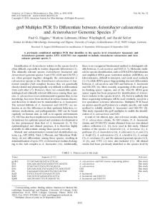
plain The area bounded by the coordinates: Latitudes :35o 22’ 00’’ S – 36o 22’ 00’’ N ; Longitudes : 41o 36’ 00’’ W – 43o 00’ 00’’ E . The Figure shows the location and the VES points distribution in the study area. The study area located to the south of the large known Sinjar anticline structure and called P
P
P
P
P
P
P
P
P
P
P
P
P
P
P
P
P
P
P
P
P
P
Sinjar plain Its surface covered with the Quarternary deposits of Pliestocene and Holocene periods, while Tertiary and cretaceous deposits are buried beneath and doesn’t expose to surface [6] .
P
P
Figure - A map showing the location, exposed to surface geological formations and VES point’s distribution within the Sinjar plain study area.
sand, silt and rarely clay. These deposits belong to Pliestocene or lower Quarternary. 3- Miqdadiyah or (lower Bakhtiari) formation deposits: It belongs to the Pliocene and a little part of early Miocene and consists of gravely sandstone, claystones and siltstones. 4- Injana or (upper Fars) formation deposits :It belongs to the middle Miocene and consists mainly of coarse grained sandstone and claystone which may exposed to surface in a relatively small spots.
The Sinjar plain area shows the following geology [7, 8]: 1- Residual soil: A Quarternary deposits of sand and locally gypsiferous loamy soil. Around sinjar anticline and almost ground level the soil shows slightly cemented rock fragments, Silt and Sand such deposits called slope deposits. 2- Terrace deposits: A Quarternary deposits exposed in some relatively small spots and composed of conglomerates with lenses of
U
U
U
U
U
U
U
360
U
Al-Yasi et .al
Iraqi Journal of Science. Vol 54.No.2.2013.Pp 358-367
5- Fatha or (lower Fars) formation deposits: It belongs to lower middle Miocene and consist of green marlstone, Limestone and gypsum. The upper member of this formation consists of red claystones and green marlstones. U
Where AB = distance between the current electrodes in meters, MN = distance between potential electrodes in meters, ∆V= potential difference measured between the potential electrodes (volts) , and I = the applied current strength. The 80 VES points were distributed on a six profiles with a midpoint interspacing of (2.5 -5), Km see figure 1. Four ground electrodes with a linear Schlumberger array achieved in the field survey where the resistivity meter (DIAPIR4000) used as a geophysical instrument. A resistivity curves drawn manually at first by making the electrode spacing values (AB/2) as an x-axis versus the apparent resistivity (ρ a ) as a y-axis on a log-log paper with a logarithmic cycle of (6.22 cm). Figure 3 The curves smoothed to solve resistivity curve discontinuities which produced by different MN spacing’s of the same AB spacing’s which is mainly caused by the lateral heterogeneity and anisotropy effect on the resistivity curve. After smoothing, resistivity curves interpreted by attending the manual (Auxiliary Point Method) of partial matching using (Orellana and Mooney, 1966) two layers Schlumberger standard curves [9]. The data also input to sophisticated computer software for VES processing and interpretation enhancement. This software used to enhance the results through the reduction of the r m s % between the calculated and the field curve as much as possible. The software uses the common forward and inversion technique [10]. figure 4,shows one of the processed and interpreted VES point No.23 by attending IpI2Win computer software. It’s important to mention that the enhancement of VES results by using such computer software’s should be attended carefully to give layers thickness as close as possible to the actual thickness values of boreholes information. The VES interpretation results represent the thickness h in meters and resistivity (ρ) in Ω.m for each of the electrical zones within each of the 80 geoelectric columns located under the midpoints of the VES points in the study area. The table 1 shows a sample of results obtained by the VES interpretation.
U
Schlumberger (VES) interpretation and results For resistivity- Hydrogeological studies, VES rofiles obtained using the Ohm resistivitymeter commonly with the Schlumberger configuration (A -M- N- B) , Figure 2 [3].
R
Figure 2- Schlumberger configuration [3].
For each (VES) point in this research study the distance between potential electrodes MN was gradually increased in steps starting from 2 m to a 100 m, according to the geometrical factor (K) for the Schlumberger configuration to obtain a measurable potential difference. The half current electrodes separation (AB/2) was usually increased in steps starting from 3.2 m to 1250 m, and the current gain (the output current) of the resistivitymeter increased gradually from 1 to 1000 mAmp., in order to increase penetration to the required depth which reached in average to 385.467m, and exceptionally to about 1000m in the VES No.30 due to the high conductivity of saline groundwater aquifer. The Schlumberger array figure 2 was used keeping the potential electrodes at a closer distance. The apparent resistivity (ρ a ) was determined using the following Equation [3]: R
R
a P
361
R
Al-Yasi et .al
Iraqi Journal of Science. Vol 54.No.2.2013.Pp 358-367
Figure 3- Profile No.3; VES No.23 manual interpretation using the auxiliary point method showing lithology obtained by the borehole K8-9 located at the middle northern part of the study area.
Figure 4- Profile No.3; VES No.23 interpretation using computer software.
361
Al-Yasi et .al
Iraqi Journal of Science. Vol 54.No.2.2013.Pp 358-367
Table 1- A sample of interpretation results of VES curves in Sinjar plain area. VES No.
ρ1
h1
ρ2
h2
ρ3
1
76.8
2.3
16.8
254
32.5
2
375
2.77
20.1
1
9.82
280
16.3
178
8.37
3
302
1.43
5.96
6.79
11.5
7.13
8.83
73.5
12.8
375
4
103
1.72
46.3
3.93
18.6
48.9
8.27
192
12
405
h3
ρ4
h4
ρ5
h5
Total Depth m
Curve Type
256.3
H
461.77
QHK
5.07
463.85
HKHK
10000
651.55
QQHA
ρ6
resistivity curves, one of them appears in the figure 3 for VES No.23. The lithologic resistivity range values for each lithologic unit in each of the six VES profiles could be simplified in table 2. By drawing the geoelectrical section for each of the VES profiles, the boreholes lithology and resistivity variation studied for each recognized lithologic unit with depth , the resistivity range for one lithologic unit (Minimum – Maximum) in each profile section is variable. Therefore, the average (Min.-Max.) resistivity value for each lithologic unit calculated for the six VES profiling lines, table 2.
The correlation between key boreholes lithologic information and the VES interpretation results of resistivity’s with depth (which are located near or at the same location), yielded a lithologic resistivity ranges table that display resistivity ranges from minimum to maximum in each of the VES profile line for every lithologic unit appears in the boreholes. There are 16 key boreholes with depth ranges between (50-570) m in the study area where lithology and depths information available and compared lately with VES
Table 2- The results of resistivity ranges (Min.-Max.) in (Ω.m) , and the average (Min.-Max.) resistivity value for each lithologic unit within the study area. Profile No.
1 Gypsiferous Loamy top soil with chert & Lst. Fragments. (Min.Max.)(Ω.m)
1 2 3 4 5 6 (Min.Max.)(Ω.m)A verage Rock resistivity range
3 Coarse grained sandstone of Injana Fn. With fresh groundwate r. (Min.Max.)(Ω.m)
4 Silty-clayey sandstone of Injana fn. With saline groundwate. (Min.Max.)(Ω.m)
5 Green Marlstone for upper Fatha Fn. Member (Min.Max.)(Ω. m)
1- 4.3 2.83 - 5 4 – 5.5 2-3 1-2 1-3
2 Terrace deposits of conglomerate with lenses of sand, silt and rarely clay. + Miqdadiyah Fn. gravely sand , claystones and siltstones.(Min.Max.) 5.94 – 16.8 5.3 – 55 7 – 9.3 10 – 50 10 - 30 10 – 20
11.4 – 32.5 11.6 – 116 9.5 – 84.1 16 – 101 22 – 71.2 13.9 - 46.4
4.15 – 9.33 5.3 – 11.6 5.7 – 9.5 3.7 – 8.8 2 – 10 3–9
0–2 0–3 2.4 – 2.5 0–2 0–1 0–1
6 Fatha Fn. Primary gypsum and Limestone . (Min.Max.)(Ω. m) 200 - ∞ 200 - ∞ 220 - ∞ 300 - ∞ 130 - ∞ 97.1 - ∞
1.97 – 3.8
8 – 30.18
14 – 75.2 fresh G. water
3.975 – 9.7 saline G. water
0.4 – 1.91
191.18 - ∞
362
Al-Yasi et .al
Iraqi Journal of Science. Vol 54.No.2.2013.Pp 358-367
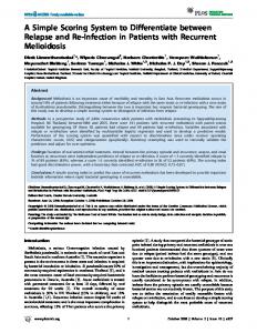
The numbers 1-6 at the most top row of table 2 refers to the lithologic unit type, these types have been drawn as an x-axis versus the rocks minimum and maximum average resistivity’s as a y- axis on a semi-log scale diagram to give a resistivity ranges comparison as it appear in figure 5.
shows the thickness variation of fresh ground water aquifer. And figure 7 shows the thickness variation of saline ground water aquifer in the study area, the data used in drawing the above mentioned figures obtained directly from the VES interpretation results. 70
60
N
50
40
30
20
10
10
20
30
40
50
60
Figure 5- A comparison diagram among (minimum & maximum) average resistivity’s for every lithologic unit within the study area .
70
80
90
100
Km Thickness (m) 520
From the comparison diagram of figure 5, there is an intermixing in the average resistivity ranges (appears highlighted with a disconnected line enclosure) that could be noticed between the lithologic unit types (2 and 3). This ranges intermixing produces an ambiguity in the VES results interpretation and make it difficult to recognize depth limits between the two types of lithologies due to the effect of equivalence and suppression. Another point worth to mention is the average resistivity range 3.975 – 9.7 for the 4th lithologic zone which represents a saline groundwater bearing zone , also, intermixes with the average resistivity range 8 – 30.18 for the 2nd lithologic zone that belongs to the fresh groundwater bearing zone, see table 2. The solution for such ambiguity solved later by the exploitation of the D-Z parameters to differentiate between fresh groundwater aquifers from those of saline ones with less ambiguity. The isolation of resistivity ranges is important to construct thickness maps for both fresh and saline groundwater bearing zones. The ranges given in the table 2, used to isolate these zones then a thickness maps showing the variation of the water-bearing zones in the study area constructed. figure 6 P
490 460
N
400 370 340 310 280 250 220 190 160 130 100 70 40 10 -20
Figure 6-The fresh groundwater aquifer thickness contour and 3D-presentation maps with a resistivity range of (10-75.2 Ω.m) for the study area, C.I. = 30 m
P
P
430
P
363
Al-Yasi et .al
Iraqi Journal of Science. Vol 54.No.2.2013.Pp 358-367
70
N
60
70
Thickness (m)
N
60
50 720
Thickness (m)
650
40
50
580 510
900 850 800 750 700 650 600 550 500 450 400 350 300 250 200 150 100 50 0 -50
40
30
20
10
10
20
30
40
50
60
70
80
90
100
30
440 370 300
20
230 160 90
10
20 -50
10
20
30
40
50
60
70
80
90
Km
Km
Thickness (m)
N N
100
720
Thickness (m)
650 580
900 850 800 750 700 650 600 550 500 450 400 350 300 250 200 150 100 50 0 -50
510 440 370 300 230 160 90 20 -50
Figure 8- The clay content thickness after subtraction of topsoil , Fresh and saline ground water aquifer thickness contour and 3D-presentation with a resistivity below 4 Ω.m for the study area , C.I. = 70 m.
Figure 7: The Saline groundwater aquifer thickness contour map and 3D-presentation with a resistivity range of (4 -9.8 Ω.m) in the study area , C.I. =50 m
.
By subtracting top soil, fresh and saline aquifers thicknesses from the whole geoelectric column thickness for every (VES) point in the area , the residual thickness obtained to represent the clay content thickness and the latter has a resistivity value equals to ,or below (4 Ω.m). Figure.8 shows the clay content thickness map in the study area.
The analysis of the D-Z parameters longitudinal unit conductance (S), transverse unit resistance (T), also, longitudinal resistivity (ρ t ) provides a very convenient and easily applicable solution to understand the geophysical behavior of saline and fresh water aquifers. (Maillet, 1947) termed the Dar Zarrouk (D-Z) parameters, figure 9. T is the resistance normal to the face and S is the conductance parallel to the face for a unit cross section area, which plays an important role in resistivity soundings (Honriet 1976 in reference [11]). R
Estimating (D-Z) parameters from (VES) results: U
As resistivities of clay with sand and saline water interfere with each other, the data interpretation becomes a difficult task. U
R
For a section consist of N fine laters with thickness h 1 , h 1 , ……. h n and resistivity ρ 1 ,ρ 2 ,…..ρ n for a block of unit square area and total thickness:
Such situation requires the formulation of better analysis technique of interpretation for the existing data to yield useful and easily understandable solution to differentiate among fresh and saline aquifers
R
R
364
R
R
R
R
R
R
R
R
R
R
Al-Yasi et .al
Iraqi Journal of Science. Vol 54.No.2.2013.Pp 358-367
The D-Z parameters have been calculated for each geoelectric column of the VES points in the Sinjar plain area according to the formula’s mentioned previously. The results used to draw up maps which appear in figures (10 to 13). It’s also possible to use the ρ t and ρ l obtained by VES interpretation results to calculate the factor of anisotropy (λ) , for every VES point geoelectric column in the study area according to the following formula that presented by (Mailet,1947), [12]:
The values of S and T are set equal to those for an isotropic block with unit square area. Therefore , the longtudinal unit conductance (S) , will be : and
R
the transverse unit resistance (T), will be:
The longtudinal resistivity, ρ l =H/S and the transverse resistivity , ρ t = T/H R
R
R
R
R
R
Where ρ t is the transverse resistivity and ρ l is the longitudinal resistivity. And the value of (λ) is mostly 2> λ >1.
R
R
R
R
R
The results of λ calculations presented as a contour map as it appears in figure 14. The λ for the study area calculated for every VES geoelectric column and all of the results gave value within the range 2> λ >1. This procedure helped to check out the calculations certainity of ρ t and ρ l . R
R
R
R
R
R
70
N
S (Mho)
60
230 215
50
200 185 170
40
155 140 125
30
110 95
Figure 9-The theory and application for the D-Z parameter in a geoelectrical column [11].
80 65
20
50 35 20
10
5 -10
The contour maps for S, T and ρ l respectively, clearly demonstrate the contour patterns of saline and fresh water aquifers over large regions with distinctly clear non intermixing boundaries and give an insight vision into the subsurface aquifer system, which can be of special importance in differentiating between fresh water aquifers and saline aquifers in some regions, it may provide a useful evidences to overcome the problem of uncertainty, caused by resistivity data interpretation [11]. R
10
R
20
30
40
50
60
70
80
90
100
Km
Figure 10- Longitudinal Conductance (S) contour map for the study area, C.I. = 15 Mho
365
Al-Yasi et .al
Iraqi Journal of Science. Vol 54.No.2.2013.Pp 358-367
70
70
N
60
50
50
47
44 42 40 38 36 34 32 30 28 26 24 22 20 18 16 14 12 10 8 6 4 2
40
30
20
10
10
20
30
40
50
60
70
80
90
40
42 37 32
30
27 22
20
17 12
10 7 2
Km Figure 13- Transverse Resistivity (ρ t ) contour map for the study area, C.I. = 5 Ω.m 10
100
Figure 11- Longitudinal Resistivity (ρ l ) contour map for the study area, C.I. = 2 Ω.m R
N
60
ρl (Ω.m)
20
30
40
50
60
70
80
90
100
R
R
R
70
70
N
60
T(Ω.m^
50
N λ
60
50
1.6 1.55
26000 24000
40
1.5
40
1.45
22000 20000
1.4
18000
30
30
1.35
16000
ρt (Ω.m)
1.3
14000
20
1.25
20
12000
1.2
10000 8000
1.15
10
6000
10
1.1
4000
1.05 2000
10
0
10
20
30
40
50
60
70
80
90
100
Km
20
30
40
50
60
70
80
90
100
Km
1
Figure 12- Transverse resistance (T) contour map for the study area, C.I. = 2000 Ω.m2
Figure 14- The factor of anisotropy (λ) contour map for the study area, C.I. = 0.05.
Conclusions: The VES interpretation results were compared with boreholes information to recognize resistivity ranges for every lithological unit in the study area, especially the fresh groundwater bearing formations and saline groundwater bearing ones, figures 6 and 7. The intermixing in resistivity range values of the above mentioned formations generated a problem that required better solution to recognize between them, this solution represented by the exploitation of D-Z geoelectric parameters. By observing D-Z contour maps, the most northern and northwestern parts of the study area yielded (S) values ranging between 5 – 50 Mho, figure 10, this referred to a relatively fresh groundwater aquifers area,
It is located adjacently to the southern limb of Sinjar anticline. This area has a ρ l range of 8 – 44 Ω.m, figure 11, ρ t range of 12 – 32Ω.m figure 13, and T range of 2000-12000 Ω.m2, figure 12 The low S value at the S-SE parts of the study area figure 10 refers to the reduction in the groundwater reservoir thickness where Fatha formation that consist of evaporates of high resistivity becomes near surface. The other parts of the study area have brackish to saline groundwater aquifers and have higher S values that ranging between 51 -230 Mho, ρ l values range of 2 –8 Ω.m, ρ t range of 2 – 12 Ω.m, and T range of 0 – 2000 Ω.m2 .
P
R
R
R
R
P
P
R
R
R
P
366
P
R
Al-Yasi et .al
Iraqi Journal of Science. Vol 54.No.2.2013.Pp 358-367
6. Daoud Y.N. 1986.application of electrical resistivity method for hydrogeological investigations in south Sinjar area. MS.C. Thesis. Department of Geology. College of Science. University of Baghdad,P.157. 7. Iraqi GEOSURV.1993.The geology of Sinjar Quadrangle. The Iraqi ministry of industry and minerals , the state establishment of geological survey and mining, GEOSURV report No.2225, NJ37-16(GM3), P.27 (unpublished) . 8. Sissakian V.K. 1995. The Geology of Mosul Quadrangle. the Iraqi ministry of industry and minerals , the state establishment of geological survey and mining GEOSURV, report No.NJ-38-3 , p.54 (unpublished) . 9. Orellana E. and Mooney H.M. 1966.Master Curves for Schlumberger Arrangement. Madrid, P.34. 10. IpI2Winv.2.1Usersguide.2001.computer software user guide catalog presented by Moscow state university, Geological faculty, Department of Geophysics and GEOSCAN-M Ltd., P.25. 11. Singh U.K. ; Das R.K. and Hodlur G.K. 2004. Significance of Dar-Zarrouk parameters in the exploration of quality affected coastal aquifer systems. Environmental Geology Springer-Verlag , 45,pp: 696–702 . 12. Mailet R. 1947. Fundamental Equations for Electrical Prospecting. Journal of Geophysics, 12,pp:528-556.
Acknowledgement The researchers appreciate the efforts of the Iraqi general commission of groundwater for the cooperation in providing the VES data and the boreholes information. Another appreciation to the Iraqi Geological Surveying and Mining Company for providing the geological information about the South Sinjar study area. References 1. George N.J.; Obianwu V.I. and Obot I.B. 2011.Estimation of groundwater reserve in unconfined frequently exploited depth of aquifer using a combined surficial geophysical and laboratory techniques in The Niger Delta, South – South, Nigeria. Pelagia Research Library (USA) AASRFC .Advances in Applied Science Research, 2(1),pp:163-177. 2. El Osta M. M.; El Sheikh A. E. and Barseem M. S. 2010. Comparative Hydrological and Geoelectrical Study on the Quaternary Aquifer in the Deltas of Wadi Badaa and Ghweiba, El Ain El Sukhna Area, Northwest Suez Gulf, Egypt. International Journal of Geophysics, (20): Article ID ,pp:15-43. 3. Batte A.G.; Muwanga A. and Sigrist W. P. 2008. Evaluating The Use Of Vertical Electrical Sounding As A Groundwater Exploration Technique To Improve On The Certainty Of Borehole Yield In Kamuli District (Eastern Uganda). African Journal of Science and Technology (AJST) Science and Engineering Series, 9(1),pp: 72 – 85. 4. Harb N.; Haddad K. and Samer F. 2010. calculations of transverse resistance to correct aquifer resistivity of groundwater saturated zones: implications for estimating its Hydrogeological properties. Lebanese Science Journal , 11(1),pp: 105-115. 5. Oseji J.O. and Ujuanbi O. 2009. Hydrogeophysical investigation of groundwater potential in Emu kingdom, Ndokwa land of Delta State, Nigeria, International Journal of Physical Sciences, 4(5),pp:.275-284.
367