Although the finite element method was extensively developed for structural and solid mechanics ... This chapter presents a summary of the basic concepts ... representation of fluid motion, it is convenient to introduce the concepts of streamlines and path lines. ..... (17.37) the application of Newton's law in x direction gives.
CHAPTER
17 ●
Basic Equations of Fluid Mechanics CHAPTER OUTLINE 17.1 Introduction 549 17.2 Basic Characteristics of Fluids 549 17.3 Methods of Describing the Motion of a Fluid 550 17.4 Continuity Equation 551 17.5 Equations of Motion or Momentum Equations 552 17.5.1 State of Stress in a Fluid 552 17.5.2 Relation between Stress and Rate of Strain for Newtonian Fluids Stress–Strain Relations for Solids 552 17.5.3 Equations of Motion 555
17.6 Energy, State, and Viscosity Equations 556 17.6.1 Energy Equation 556 17.6.2 State and Viscosity Equations 557
17.7 17.8 17.9 17.10 17.11 17.12
Solution Procedure 557 Inviscid Fluid Flow 559 Irrotational Flow 560 Velocity Potential 561 Stream Function 562 Bernoulli Equation 564
17.1 INTRODUCTION Although the finite element method was extensively developed for structural and solid mechanics problems, it was not considered a powerful tool for the solution of fluid mechanics problems until recently. One of the reasons is the success achieved with the more traditional finite difference procedures in solving fluid flow problems. In recent years, significant contributions have been made in the solution of different types of fluid flow problems using the finite element method. This chapter presents a summary of the basic concepts and equations of fluid mechanics.
17.2 BASIC CHARACTERISTICS OF FLUIDS A fluid is a substance (gas or liquid) that will deform continuously under the action of applied surface (shearing) stresses. The magnitude of the stress depends on the rate of angular deformation. On the other hand, a solid can be defined as a substance that will deform by an amount proportional to the stress applied after which static equilibrium will result. Here, the magnitude of the shear stress depends on the magnitude of angular deformation.
The Finite Element Method in Engineering. DOI: 10.1016/B978-1-85617-661-3.00017-9 © 2011 Elsevier Inc. All rights reserved.
549
PART 5 Application to Fluid Mechanics Problems Different fluids show different relations between stress and the rate of deformation. Depending on the nature of relation followed between stress and rate of deformation, fluids can be classified as Newtonian and non-Newtonian fluids. A Newtonian fluid is one in which the shear stress is directly proportional to the rate of deformation starting with zero stress and zero deformation. The constant of proportionality is defined as μ, the absolute or dynamic viscosity. Common examples of Newtonian fluids are air and water. A non-Newtonian fluid is one that has a variable proportionality between stress and rate of deformation. Common examples of non-Newtonian fluids are some plastics, colloidal suspensions, and emulsions. Fluids can also be classified as compressible and incompressible. Usually, liquids are treated as incompressible, whereas gases and vapors are assumed to be compressible. A flow field is described in terms of the velocities and accelerations of fluid particles at different times and at different points throughout the fluid-filled space. For the graphical representation of fluid motion, it is convenient to introduce the concepts of streamlines and path lines. A streamline is an imaginary line that connects a series of points in space at a given instant in such a manner that all particles falling on the line at that instant have velocities whose vectors are tangent to the line. Thus, the streamlines represent the direction of motion at each point along the line at the given instant. A path line is the locus of points through which a fluid particle of fixed identity passes as it moves in space. For a steady flow the streamlines and path lines are identical, whereas they are, in general, different for an unsteady flow.
550
A flow may be termed as inviscid or viscous depending on the importance of consideration of viscosity of the fluid in the analysis. An inviscid flow is a frictionless flow characterized by zero viscosity. A viscous flow is one in which the fluid is assumed to have nonzero viscosity. Although no real fluid is inviscid, there are several flow situations in which the effect of viscosity of the fluid can be neglected. For example, in the analysis of a flow over a body surface, the viscosity effects are considered in a thin region close to the flow boundary (known as boundary layer), whereas the viscosity effect is neglected in the rest of the flow. Depending on the dynamic macroscopic behavior of the fluid flow, we have laminar, transition, and turbulent motion. A laminar flow is an orderly state of flow in which macroscopic fluid particles move in layers. A turbulent flow is one in which the fluid particles have irregular, fluctuating motions and erratic paths. In this case, macroscopic mixing occurs both lateral to and in the direction of the main flow. A transition flow occurs whenever a laminar flow becomes unstable and approaches a turbulent flow.
17.3 METHODS OF DESCRIBING THE MOTION OF A FLUID The motion of a group of particles in a fluid can be described by either the Lagrangian method or the Eulerian method. In the Lagrangian method, the coordinates of the moving particles are represented as functions of time. This means that at some arbitrary time t0, the coordinates of a particle (x0, y0, z0) are identified and that thereafter we follow that particle through the fluid flow. Thus, the position of the particle at any other instant is given by a set of equations of the form x = f1 ðx0 , y0 , z0 , t Þ,
y = f2 ðx0 , y0 , z0 , t Þ,
z = f3 ðx0 , y0 , z0 , t Þ
The Lagrangian approach is not generally used in fluid mechanics because it leads to more cumbersome equations. In the Eulerian method, we observe the flow characteristics in the vicinity of a fixed point as the particles pass by. Thus, in this approach the velocities at various points are expressed as functions of time as u = f1 ðx, y, z, t Þ,
v = f2 ðx, y, z, t Þ,
w = f3 ðx, y, z, t Þ
where u, v, and w are the components of velocity in x, y, and z directions, respectively.
CHAPTER 17 Basic Equations of Fluid Mechanics The velocity change in the vicinity of a point in the x direction is given by du =
∂u ∂u ∂u ∂u dt + dx + dy + dz ∂t ∂x ∂y ∂z
(17.1)
(total derivative expressed in terms of partial derivatives). The small distances moved by a particle in time dt can be expressed as dx = u dt,
dy = v dt,
dz = w dt
(17.2)
Thus, dividing Eq. (17.1) by dt and using Eq. (17.2) leads to the total or substantial derivative of the velocity u (x component of acceleration) as ax = du ≡ Du = ∂u + u ∂u + v ∂u + w ∂u dt Dt ∂t ∂x ∂y ∂z
(17.3a)
The other components of acceleration can be expressed in a similar manner as ay =
dv ≡ Dv = ∂v + u ∂v + v ∂v + w ∂v dt Dt ∂t ∂x ∂y ∂z
(17.3b)
az = dw ≡ Dw = ∂w + u ∂w + v ∂w + w ∂w dt Dt ∂t ∂x ∂y ∂z
(17.3c)
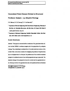
17.4 CONTINUITY EQUATION To derive the continuity equation, consider a differential control volume of size dx dy dz as shown in Figure 17.1. Assuming that the density and the velocity are functions of space and time, we obtain the flux of mass per second for the three directions x, y, and z, respectively, ∂ ∂ ∂ as − ðρuÞ ⋅ dy dz, − ðρvÞ ⋅ dx dz, and − ðρwÞ ⋅ dx dy. From the principle of conservation ∂x ∂y ∂z ∂ of matter, the sum of these must be equal to the time rate of change of mass, ðρdx dy dzÞ. ∂t
dy ρu +
[ρu] dy dz
y dz dx
x
z
FIGURE 17.1 Differential Control Volume for Conservation of Mass.
∂ (ρu ) dx dy dz ∂x
551
PART 5 Application to Fluid Mechanics Problems Since the control volume is independent of time, we can cancel dx dy dz from all the terms and obtain ∂ρ + ∂ ðρuÞ + ∂ ðρvÞ + ∂ ðρwÞ = 0 ∂t ∂x ∂y ∂z
(17.4a)
where ρ is the mass density; u, v, and w are the x, y, and z components of velocity, respectively; and t is time. By using the vector notation ! ! ! ! V = u i + v j + wk = velocity vector and ! ∂! ∂! ∂! i + j + k = gradient vector ∇= ∂x ∂y ∂z ! ! ! where i , j , and k represent the unit vectors in x, y, and z directions, respectively. Equation (17.4a) can be expressed as ∂ρ ! ! + ∇ ⋅ ρ∇ = 0 ∂t
(17.4b)
∂u + ∂v + ∂w = − 1 DðρÞ ∂x ∂y ∂z ρ Dt
(17.4c)
This equation can also be written as
where (D/Dt) represents the total or substantial derivative with respect to time. Equations (17.4) represents the general three-dimensional continuity equation for a fluid in unsteady flow. If the fluid is incompressible, the time rate of volume expansion of a fluid element will be zero and hence the continuity equation, for both steady and unsteady flows, becomes ! ! ∂u ∂v ∂w ∇⋅V = + + =0 ∂x ∂y ∂z
552
(17.5)
17.5 EQUATIONS OF MOTION OR MOMENTUM EQUATIONS 17.5.1 State of Stress in a Fluid The state of stress in a fluid is characterized, as in the case of a solid, by the six stress components σ xx , σ yy , σ zz , σ xy , σ yz , and σ zx : However, if the fluid is at rest, the shear stress components σ xy , σ yz , and σ zx will be zero and all the normal stress components will be the same and equal to the negative of the hydrostatic pressure, p—that is, σ xx = σ yy = σ zz = −p:
17.5.2 Relation between Stress and Rate of Strain for Newtonian Fluids STRESS–STRAIN RELATIONS FOR SOLIDS In solids the stresses σ ij are related to the strains εij according to Hooke’s law, Eq. (8.7): 9 1 = εxx = ½σ xx − νðσ yy + σ zz Þ�, … > E (17.6) σ xy > ; ,… εxy = G If an element of solid having sides dx, dy, and dz is deformed into an element having sides ð1 + εxx Þdx, ð1 + εyy Þdy, and ð1 + εzz Þdz, the volume dilation of the element (e) is defined as e=
change in volume of the element original volume of the element
ð1 + εxx Þð1 + εyy Þð1 + εzz Þdx dy dz − dx dy dz dx dy dz = εxx + εyy + εzz =
(17.7)
CHAPTER 17 Basic Equations of Fluid Mechanics Using Eq. (17.6), Eq. (17.7) can be expressed as e=
1 − 2v 1 − 2v ðσ xx + σ yy + σ zz Þ = 3σ E e
(17.8)
where σ is the arithmetic mean of the three normal stresses defined as σ = ðσ xx + σ yy + σ zz Þ/3
(17.9)
Young’s modulus and Poisson’s ratio are related as G=
E E or 2G = 2ð 1 + v Þ 1+v
(17.10)
The first equation of Eq. (17.6) can be rewritten as εxx =
1 E 3v ½σ xx − vðσ xx + σ yy + σ zz Þ + vσ xx � = εxx + σ E 1+v 1+v
(17.11)
Substituting for 3σ from Eq. (17.9) into Eq. (17.11) and using the relation (17.10), we obtain σ xx =
E ε v E ⋅ e = 2Gε 2Gv ⋅ e xx + xx + 1+v 1 + v 1 − 2v 1 − 2v
(17.12)
By subtracting σ from both sides of Eq. (17.12) we obtain σ xx − σ = 2Gεxx +
2Gv e−σ 1 − 2v
(17.13)
Using Eq. (17.8), Eq. (17.13) can be expressed as E e σ xx − σ = 2Gεxx + 2Gv e − 1 − 2v 3ð1 − 2vÞ that is,
� � e σ xx − σ = 2Gεxx − 3
In a similar manner, the following relations can be derived: � � e σ yy − σ = 2G εyy − 3 � � e σ zz − σ = 2G εzz − 3
553
(17.14)
(17.15) (17.16)
The shear stress–shear strain relations can be written, from Eq. (17.6), as σ xy = Gεxy
(17.17)
σ yz = Gεyz
(17.18)
σ zx = Gεzx
(17.19)
STRESS–RATE OF STRAIN RELATIONS FOR NEWTONIAN FLUIDS Experimental results indicate that the stresses in a fluid are related to the time rate of strain instead of strain itself. Thus, the stress–rate of strain relations can be derived by analogy from Eqs. (17.14) to (17.19). As an example, consider Eq. (17.14). By replacing the shear modulus (G) by a quantity expressing its dimensions, we obtain � � �� F e (17.20) σ xx − σ = 2 2 εxx − L 3
PART 5 Application to Fluid Mechanics Problems where F is the force, and L is the length. Since the stresses are related to the time rates of strain for a fluid, Eq. (17.20) can be used to obtain the following relation valid for a Newtonian fluid: � � � � FT ∂ e εxx − σ xx − σ = 2 2 (17.21) L ∂t 3 In Eq. (17.21), the dimension of time (T) is added to the proportionality constant in order to preserve the dimensions. The proportionality constant in Eq. (17.21) is taken as the dynamic viscosity µ having dimensions FT/L2. Thus, Eq. (17.21) can be expressed as
554
σ xx − σ = 2μ
∂εxx 2 ∂e − ∂t 3 ∂t
(17.22)
σ yy − σ = 2μ
∂εyy 2 ∂e − ∂t 3 ∂t
(17.23)
σ zz − σ = 2μ
∂εzz 2 ∂e − 3 ∂t ∂t
(17.24)
σ xy = μεxy
(17.25)
σ yz = μεyz
(17.26)
σ zx = μεzx
(17.27)
If the coordinates of a point before deformation are given by x, y, z and after deformation by x + ξ, y + η, z + ζ, the strains are given by 9 ∂η ∂ξ ∂ζ > , εzz = , εyy = εxx = > = ∂y ∂x ∂z (17.28) ∂η ∂ζ ∂ξ ∂η ∂ζ ∂ξ > ; + , εzx = + , εyz = + > εxy = ∂z ∂y ∂y ∂x ∂x ∂z The rate of strain involved in Eq. (17.22) can be expressed as � � � � ∂εxx ∂ ∂ξ ∂ ∂ξ ∂u = = = ∂t ∂t ∂x ∂x ∂t ∂x where u is the component of velocity in x direction, and � ∂u ∂v ∂w ! ! ∂e ∂� = εxx + εyy + εzz = + + = ∇⋅V ∂t ∂t ∂x ∂y ∂z
(17.29)
(17.30)
The mean stress σ is generally taken as −p, where p is the mean fluid pressure. Thus, Eqs. (17.22) to (17.27) can also be expressed as ∂u 2 ! ! (17.31) σ xx = −p + 2μ − μ ∇ ⋅ V ∂x 3 σ yy = −p + 2μ
! ∂v − 2 μ! ∇⋅V ∂y 3
∂w 2 ! ! − μ∇ ⋅ V ∂z 3 � � ∂v + ∂u σ xy = μ ∂x ∂y
σ zz = −p + 2μ
� � σ yz = μ ∂w + ∂v ∂y ∂z σ zx = μ
�
∂u + ∂w ∂z ∂x
�
(17.32) (17.33) (17.34) (17.35) (17.36)
CHAPTER 17 Basic Equations of Fluid Mechanics
17.5.3 Equations of Motion The equations of motion can be derived by applying Newton’s second law to a differential volume (dx dy dz) of a fixed mass dm [17.1]. If the body forces acting on the fluid per unit mass are given by the vector ! ! ! ! (17.37) B = Bx i + By j + Bz k the application of Newton’s law in x direction gives dFx = dm ax = ðρ dx dy dzÞax
(17.38)
where dFx is the differential force acting in x direction, and ax is the acceleration of the fluid in x direction. Using a figure similar to that of Figure 8.2, Eq. (17.38) can be rewritten as � � ∂σ dFx = ðρdx dy dzÞBx − σ xx dy dz + σ xx + xx dx dy dz − σ yx dx dz ∂x � � � � ∂σ yx ∂σ dy dx dz − σ zx dx dy + σ zx + zx dz dx dy + σ yx + ∂y ∂z Dividing this equation throughout by the volume of the element gives ρBx +
∂σ xx ∂σ yx ∂σ zx + + = ρax ∂x ∂y ∂z
(17.39a)
Similarly, we can obtain for the y and z directions, ρBy +
∂σ xy ∂σ yy ∂σ zy + + = ρay ∂x ∂y ∂z
(17.39b)
ρBz +
∂σ xz ∂σ yz ∂σ zz + + = ρaz ∂x ∂y ∂z
(17.39c)
Equations (17.39) are general and are applicable to any fluid with gravitational-type body forces. For Newtonian fluids with a single viscosity coefficient, we substitute Eqs. (17.31) to (17.36) into Eqs. (17.39) and obtain the equations of motion in x, y, and z directions as � � � � h � �i ∂p ! !� ∂ ∂ ∂u 2 ∂v ∂u + ρax = ρBx − 2μ − μ ∇ ⋅ V + μ + + ∂ μ ∂u + ∂w (17.40a) ∂x ∂x ∂x 3 ∂y ∂x ∂y ∂z ∂z ∂x ρay = ρBy −
� � � � � � � � ∂p ! ∂ μ ∂u + ∂v + ∂ 2μ ∂v − 2 μ! ∇ ⋅ V + ∂ μ ∂v + ∂w + ∂y ∂x ∂y ∂y 3 ∂z ∂z ∂y ∂y ∂x
(17.40b)
� � � � � � � � ∂p ! ∂ μ ∂w + ∂u + ∂ μ ∂v + ∂w + ∂ 2μ ∂w − 2 μ! ∇⋅V (17.40c) + ∂x ∂z ∂y ∂z ∂y ∂z ∂z 3 ∂z ∂x ︸ |{z} ︸ |fflfflfflfflfflfflfflfflfflfflfflfflfflfflfflfflfflfflfflfflfflfflfflfflfflfflfflfflfflfflfflfflfflfflfflfflfflfflfflfflfflfflfflfflfflfflfflfflfflfflfflfflfflfflfflffl{zfflfflfflfflfflfflfflfflfflfflfflfflfflfflfflfflfflfflfflfflfflfflfflfflfflfflfflfflfflfflfflfflfflfflfflfflfflfflfflfflfflfflfflfflfflfflfflfflfflfflfflfflfflfflfflffl}︸ |{z} ︸ |{z} Viscous force Inertia Body Pressure force force force ρaz = ρBz −
Equations (17.40) are called the Navier-Stokes equations for compressible Newtonian fluids in Cartesian form. For incompressible fluids, the Navier-Stokes equations of motion, Eqs. (17.40), become � � ∂p μ ∂2 u ∂2 u ∂2 u ax = ∂u + u ∂u + v ∂u + w ∂u = Bx − 1 + (17.41a) + + ∂t ∂x ∂y ∂z ρ ∂x ρ ∂x2 ∂y2 ∂z2 � � ∂v ∂v ∂v ∂v 1 ∂p μ ∂2 v ∂2 v ∂2 v + ay = (17.41b) + + +u +v +w = By − ∂t ∂x ∂y ∂z ρ ∂y ρ ∂x2 ∂y2 ∂z2 � � ∂w ∂w ∂w ∂w 1 ∂p μ ∂2 w ∂2 w ∂2 w + az = (17.41c) + + +u +v +w = Bz − ∂t ∂x ∂y ∂z ρ ∂z ρ ∂x2 ∂y2 ∂z2
555
PART 5 Application to Fluid Mechanics Problems Furthermore, when viscosity µ is zero, Eqs. (17.41) reduce to the Euler equations: a x = Bx −
1 ∂p ρ ∂x
(17.42a)
ay = By −
1 ∂p ρ ∂y
(17.42b)
a z = Bz −
1 ∂p ρ ∂z
(17.42c)
For steady flow, all derivatives with respect to time will be zero in Eqs. (17.40) to (17.42).
17.6 ENERGY, STATE, AND VISCOSITY EQUATIONS 17.6.1 Energy Equation When the flow is nonisothermal, the temperature of the fluid will be a function of x, y, z, and t. Just as the continuity equation represents the law of conservation of mass and gives the velocity distribution in space, the energy equation represents the conservation of energy and gives the temperature distribution in space. To derive the energy equation, we consider a differential control volume of fluid of size dx dy dz and write the energy balance equation as Energy input = energy output + energy accumulation
556
(17.43)
The energy input to the element per unit time is given by �n o n o ∂ dx 1 ρuðu2 2 ∂ dx ρuE − ðρuEÞ ⋅ + v + w2 Þ − ½ ρuðu2 + v2 + w2 Þ� ⋅ + ∂x 2 2 |fflfflfflfflfflfflfflfflfflfflfflfflfflfflfflfflfflfflfflfflfflfflfflfflfflfflfflfflfflfflfflfflfflfflfflfflfflfflfflfflfflffl ∂xffl{zfflfflfflfflfflfflfflfflfflfflfflfflfflfflfflfflfflfflfflfflfflfflfflfflfflfflfflfflfflfflfflfflfflfflfflfflfflfflfflfflfflffl 2 ffl} |fflfflfflfflfflfflfflfflfflfflfflfflfflfflfflfflfflffl{zfflfflfflfflfflfflfflfflfflfflfflfflfflfflfflfflfflffl} ︸ ︸ Internal energy Kinetic energy n o n � � o ∂ ðpuÞ dx ∂T − ∂ k ∂T dx ︸ ⋅ dydz + pu − ︸ − k ⋅ ∂x 2 ffl} ∂x ∂xffl{zfflfflfflfflfflfflfflfflfflfflfflfflfflfflfflfflfflfflfflffl ∂x 2 ffl} |fflfflfflfflfflfflfflfflfflfflfflfflfflfflfflfflfflfflfflffl |fflfflfflfflfflfflfflfflfflfflfflfflfflffl ffl{zfflfflfflfflfflfflfflfflfflfflfflfflfflffl Heat conduction Pressure–volume work + similar terms for y and z directions +
∂Q dx dy dz + Φ dx dy dz ∂t
where T is the temperature, k is the thermal conductivity, Q is the heat generated in the fluid per unit volume, and Φ is the dissipation function—that is, time rate of energy dissipated per unit volume due to the action of viscosity. Similarly, the energy output per unit time is given by �h i n o � ∂ � 2 2 �� ∂ dx 1 ρu�u2 ρu u + v + w2 ⋅ dx ρuE + ðρuEÞ ⋅ + v 2 + w2 + + ∂x 2 2 ∂x 2 h i n � � o ∂ dx ∂T ∂ ∂T dx + pu + ðpuÞ + k − k ⋅ ⋅ dy dz ∂x 2 ∂x ∂x ∂x 2 + similar terms for y and z directions The energy accumulated in the element is given by � � � 2 �� ∂ 1 ∂ 2 2 + dx dy dz ðρEÞ︸ ρ u +v +w ∂x 2 ∂t |fflfflfflffl{zfflfflfflffl} |fflfflfflfflfflfflfflfflfflfflfflfflfflfflfflffl{zfflfflfflfflfflfflfflfflfflfflfflfflfflfflfflffl} Internal energy ︸Kinetic energy
(17.44)
CHAPTER 17 Basic Equations of Fluid Mechanics By making the energy balance as per Eq. (17.43), we obtain, after some manipulation, � � � � � � ∂Q ∂ ∂T ∂ ∂T ∂ ∂T +Φ k k + k + + ∂t ∂x ∂x ∂y ∂y ∂z ∂z (17.45) DðEÞ ρ D 2 2 ∂ ∂ ∂ 2 = ðpuÞ + ðpvÞ + ðpwÞ + ðu + v + w Þ + ρ Dt 2 Dt ∂x ∂y ∂z By using the relation
� ∂E � = specific heat at constant volume � ∂T at constant volume DðEÞ DT in place of we can substitute cv ⋅ in Eq. (17.45). Dt Dt ! ! For inviscid and incompressible fluids, ∇ ⋅ V = 0, and the application of Eq. (17.43) leads to cv =
∂Q DT +Φ (17.46) = k∇2 T + ∂t Dt where cv is the specific heat at constant volume, T is the temperature, k is the thermal conductivity, Q is the heat generated in the fluid per unit volume, and Φ is the dissipation function (i.e., time rate of energy dissipated per unit volume due to the action of viscosity) [17.2] given by " # � �2 � �2 � �2 � �2 2 ∂u ∂v ∂w ∂u ∂v ∂w Φ= − μ + 2μ + + + + 3 ∂x ∂y ∂z ∂x ∂y ∂z "� # (17.47) �2 � � � 2 � ∂w ∂v ∂u ∂w 2 ∂v ∂u +μ + + + + + ∂y ∂z ∂z ∂x ∂x ∂y ρcv
It can be seen that Φ has a value of zero for inviscid fluids. 557
17.6.2 State and Viscosity Equations The variations of density and viscosity with pressure and temperature can be stated in the form of equations of state and viscosity as ρ = ρðp, T Þ
(17.48)
μ = μðp, T Þ
(17.49)
17.7 SOLUTION PROCEDURE For a general three-dimensional flow problem, the continuity equation, the equations of motion, the energy equation, the equation of state, and the viscosity equation are to be satisfied. The unknowns are the velocity components (u, v, w), pressure (p), density (ρ), viscosity (µ), and the temperature (T). Thus, there are seven governing equations in seven unknowns, and hence the problem can be solved once the flow boundaries and the boundary and initial conditions for the governing equations are known. The general governing equations are valid at any instant of time and are applicable to laminar, transition, and turbulent flows. Note that the solution of the complete set of equations has not been obtained even for laminar flows. However, in many practical situations, the governing equations get simplified considerably, and hence the mathematical solution would not be very difficult. In a turbulent flow, the unknown variables fluctuate about their mean values randomly and the solution of the problem becomes extremely complex. For a three-dimensional inviscid fluid flow, five unknowns, namely, u, v, w, p, and ρ, will be there. In this case, Eqs. (17.4) and (17.40) are used along with the equation of state (expressing ρ in terms of pressure p only) to find the unknowns. In the solution of these equations, constants of integration appear that must be evaluated from the boundary conditions of the specific problem.
PART 5 Application to Fluid Mechanics Problems
EXAMPLE 17.1 Express the Navier-Stokes equations for the flow of an incompressible Newtonian fluid.
Solution For an incompressible Newtonian fluid, the stresses vary linearly with the rate of deformation so that the normal stresses are given by σ xx = −p + 2μ ∂u , ∂x and the shear stresses by σ xy = σ yx = μ
� � ∂u ∂v + , ∂y ∂x
σ yy = −p + 2μ ∂v , ∂y
σ zz = −p + 2μ ∂w ∂z
� � ∂v ∂w σ yz = σ zy = μ + , ∂z ∂y
σ zx = σ xz = μ
�
(E.1)
� ∂w ∂u + ∂x ∂z
(E.2)
By substituting Eqs. (E.1) and (E.2) and the expressions for the acceleration components of the fluid given by Eqs. (17.3) into the equations of motion (obtained by considering the dynamic equilibrium of a small cube-type of element) given by Eqs. (17.39), we obtain the equations of motion (Navier-Stokes equations) in the x, y, and z directions (for incompressible flow of a Newtonian fluid) as � � � � ∂p ∂u ∂u ∂u ∂u ∂2 u ∂2 u ∂2 u ρ +u +v +w = − + ρ Bx + μ + 2 + 2 (E.3) 2 ∂t ∂x ∂y ∂z ∂x ∂y ∂z ∂x � � � � ∂p ∂v ∂v ∂v ∂v ∂2 v ∂2 v ∂2 v +u +v +w = − + ρ By + μ + + ∂t ∂x ∂y ∂z ∂x2 ∂y2 ∂z2 ∂y
(E.4)
� � � � ∂p ∂w ∂w ∂w ∂w ∂2 w ∂2 w ∂2 w +u +v +w + + ρ = − + ρ Bz + μ ∂t ∂x ∂y ∂z ∂x2 ∂y2 ∂z2 ∂z
(E.5)
ρ
558
EXAMPLE 17.2 Find an expression for the velocity of the fluid in a steady laminar flow between two fixed parallel plates.
Solution Let the fluid flow between the parallel plates shown in Figure 17.2(a). Here a fluid particle moves in the x direction parallel to the plate, and hence it has no velocity in the y or z direction so that v = w = 0. Thus, the continuity equation, Eq. (17.5), becomes
y y
h
u x
u(y )
0
x
h
(a) Viscous fluid flow between parallel plates
(b) Velocity distribution in y direction
FIGURE 17.2 Viscous Fluid Flow between Parallel Plates. ∂u = 0 ∂x
(E.1)
In addition, there is no variation of u in the z direction by assuming the plates to be infinite in the z direction. For steady flow, ∂u = 0 ∂t
CHAPTER 17 Basic Equations of Fluid Mechanics
Thus, u can be expressed as u = uðyÞ
(E.2)
Using these conditions, the Navier-Stokes equations given by Eqs. (E.3) to (E.5) of Example 17.1 reduce to −
∂p ∂2 u +μ 2 = 0 ∂y ∂x
(E.3)
∂p −ρg = 0 ∂y
(E.4)
∂p =0 ∂z
(E.5)
−
−
where Bx = 0, By = −g, Bz = 0 have been assumed (g = acceleration due to gravity). Equations (E.4) and (E.5) can be integrated to obtain p = −ρ g y + f ðxÞ
(E.6)
where f(x) is some function of x. By rewriting Eq. (E.3) as ∂2 u 1 ∂p = ∂y2 μ ∂x and assuming
∂p to be a constant, Eq. (E.7) can be integrated to obtain ∂x ∂u 1 ∂p = y + c1 ∂y μ ∂x
(E.7)
(E.8)
where c1 is a constant of integration. Integration of Eq. (E.8) yields u=
� � 1 ∂p 2 y + c1 y + c2 2μ ∂x
(E.9)
where c2 is another constant of integration. Because the plates are fixed, u = 0 at y = +h and –h. Using these boundary conditions in Eq. (E.9), we find the values of the constants as � � ∂p 2 h c1 = 0, c2 = − 1 (E.10) 2μ ∂x Thus, the velocity of the fluid flowing between the parallel plates is given by u=
� � � 1 ∂p � 2 y − h2 2μ ∂x
(E.11)
The variation of the velocity u in the y direction is shown in Figure 17.2(b).
17.8 INVISCID FLUID FLOW In a large number of fluid flow problems (especially those with low-viscosity fluids, such as water and the common gases), the effect of viscosity will be small compared to other quantities, such as pressure, inertia force, and field force; hence, the fluid can be treated as an inviscid fluid. Typical problems in which the effect of viscosity of the fluid can be neglected are flow through orifices, flow over weirs, flow in channel and duct entrances, and flow in converging and diverging nozzles. In these problems, the conditions very near the solid boundary, where the viscosity has a significant effect, are not of much interest and one would normally be interested in the movement of the main mass of the fluid. In any fluid flow problem, we would be interested in determining the fluid velocity and fluid pressure as a function of spatial coordinates and time. This solution will be greatly simplified if the viscosity of the fluid is assumed to be zero.
559
PART 5 Application to Fluid Mechanics Problems The equations of motion (Euler’s equations) for this case are 9 Du ∂u ∂u ∂u ∂u 1 ∂p > > = +u +v +w = Bx − > Dt ∂t ∂x ∂y ∂z ρ ∂x > > > = ∂p Dv = ∂v + u ∂v + v ∂v + w ∂v = B − 1 y Dt ∂t ∂x ∂y ∂z ρ ∂y > > > > Dw ∂w ∂w ∂w ∂w 1 ∂p > > ; = +u +v +w = Bz − Dt ∂t ∂x ∂y ∂z ρ ∂z
(17.50)
The continuity equation is given by Eq. (17.4). Thus, the unknowns in Eqs. (17.50) and (17.4) are u, v, w, p, and ρ. Since the density ρ can be expressed in terms of the pressure p by using the equation of state, the four equations represented by Eqs. (17.50) and (17.4) are sufficient to solve for the four unknowns u, v, w, and p. While solving these equations, the constants of integration that appear are to be evaluated from the boundary conditions of the specific problem.
17.9 IRROTATIONAL FLOW Let a point A and two perpendicular lines AB and AC be considered in a two-dimensional fluid flow. These lines, which are fixed to the fluid, are assumed to move with the fluid and assume the positions A’B’ and A’C’ after time Dt as shown in Figure 17.3. If the original lines AB and AC are taken parallel to the x and y axes, the angular rotation of the fluid immediately adjacent to point A is given by 1 ðβ1 + β2 Þ, and hence the rate of rotation of 2 the fluid about the z axis (ωz) is defined as ωz =
1 β1 + β2 2 Δt
(17.51)
If the velocities of the fluid at the point A in x and y directions are u and v, respectively, the velocity components of the point C are u + ð∂u/∂yÞ ⋅ Δy and v + ð∂v/∂yÞ ⋅ Δy in x and y directions, respectively, where Dy = AC. Since β2 is small, � � ∂u uΔt − u + Δy Δt ∂y C’C2 A A’ − CC1 = − ∂u Δt (17.52) tan β2 = β2 = = 1 = Δy ∂y A’C2 A’C2
560
where it was assumed that A’C2 ≈ AC = Dy. Similarly, � � ∂v v + Δx Δt − vΔt B B’ ∂v Δt ∂x tan β1 = β1 = 1 = = ∂x A’B1 Δx Thus, the rate of rotation (also called rotation) can be expressed as 0∂v 1 � � Δt − ∂u Δt ∂y C 1 ∂v ∂u 1 B∂x − ωz = @ A= 2 2 ∂x ∂y Δt
FIGURE 17.3 Angular Rotation of Fluid. C′
C2
C C 1 β2 B2 Δy A1
B′
β1
B1
A′
y A x
Δx
B
(17.53)
(17.54)
By proceeding in a similar manner, the rates of rotation about the x, y, and z axes in a three-dimensional fluid flow can be derived as � � 1 ∂w − ∂v (17.55a) ωx = 2 ∂y ∂z � � 1 ∂u − ∂w 2 ∂z ∂x � � 1 ∂v − ∂u ωz = 2 ∂x ∂y ωy =
(17.55b) (17.55c)
CHAPTER 17 Basic Equations of Fluid Mechanics
(a)
(b)
FIGURE 17.4 Irrotational and Rotational Flows.
When the particles of the fluid are not rotating, the rotation is zero and the fluid is called irrotational. The physical meaning of irrotational flow can be seen in Figure 17.4. In Figure 17.4(a), the particle maintains the same orientation everywhere along the streamline without rotation. Hence, it is called irrotational flow. On the other hand, in Figure 17.4(b), the particle rotates with respect to fixed axes and maintains the same orientation with respect to the streamline. Hence, this flow is not irrotational. The vorticity or fluid rotation � � vector ! ω is defined as the average angular velocity of any two mutually perpendicular line segments of the fluid whose x, y, and z components are given by Eq. (17.55).
NOTE In both Figures 17.4(a) and 17.4(b), the particles can undergo deformation without affecting the analysis. For example, in the flow of a nonviscous fluid between convergent boundaries, the elements of the fluid deform as they pass through the channel, but there is no rotation about the z axis as shown in Figure 17.5.
561 A′
A
Streamlines
FIGURE 17.5 Irrotational Flow between Convergent Boundaries.
17.10 VELOCITY POTENTIAL It is convenient to introduce a function ϕ, called the potential function or velocity potential, in integrating Eqs. (17.50). This function ϕ is defined in such a way that its partial derivative in any direction gives the velocity in that direction; that is, ∂ϕ = u, ∂x
∂ϕ = v, ∂y
∂ϕ =w ∂z
Substitution of Eqs. (17.56) into Eq. (17.4) gives � 2 � ∂ ϕ ∂2 ϕ ∂2 ϕ ∂ρ ∂ρ ∂ρ ∂ρ Dρ −ρ = = u +v +w + + + ∂x2 ∂y2 ∂z2 ∂x ∂y ∂z ∂t Dt
(17.56)
(17.57)
For incompressible fluids, Eq. (17.57) becomes ∇2 ϕ =
∂2 ϕ ∂2 ϕ ∂2 ϕ + 2 + 2 =0 ∂x2 ∂y ∂z
(17.58)
PART 5 Application to Fluid Mechanics Problems By differentiating u and v with respect to y and x, respectively, we obtain ∂2 ϕ ∂u = , ∂y ∂y∂x
∂2 ϕ ∂v = ∂x ∂x∂y
(17.59)
from which we can obtain ∂u ∂v − =0 ∂y ∂x
(17.60)
∂u − ∂w = 0 ∂z ∂x
(17.61)
∂w ∂v − =0 ∂y ∂z
(17.62)
The terms on the left-hand side of Eqs. (17.60) to (17.62) can be seen to be equal to twice the rates of rotation of the fluid element. Thus, the assumption of a velocity potential defined by Eq. (17.56) requires the flow to be irrotational.
17.11 STREAM FUNCTION The motion of the fluid, at every point in space, can be represented by means of a velocity vector showing the direction and magnitude of the velocity. Since representation by vectors is unwieldy, we can use streamlines, which are the lines drawn tangent to the velocity vector at every point in space. Since the velocity vectors meet the streamlines tangentially for all points on a streamline, no fluid can cross the streamline. For a two-dimensional flow, the streamlines can be represented in a two-dimensional plane. A stream function ψ may be defined (which is related to the velocity of the fluid) on the basis of the continuity equation and the nature of the streamlines. Let the streamlines AB and CD denote the stream functions ψ1 and ψ2, respectively, in Figure 17.6. If a unit thickness of the fluid is considered, ψ2 – ψ1 is defined as the volume rate of fluid flow between the streamlines AB and CD. Let the streamline C’D’ lie at a small distance away from CD and let the flow between the streamlines CD and C’D’ be dψ. At a point P on CD, the distance between CD and C’D’ is denoted by the components of distance –dx and dy. Let the velocity of the fluid at point P be u and v in x and y directions, respectively. Since no fluid crosses the streamlines, the volume rate of flow across the element dy is u dy and the volume rate of flow across the element –dx is –v dx. If the flow is assumed to be incompressible, this volume rate of flow must be equal to dψ
562
∴ dψ = u dy = −v dx
(17.63)
Because ψ is a function of both x and y, we use partial derivatives and rewrite Eq. (17.63) as ∂ψ = u, ∂y FIGURE 17.6 Stream Lines Corresponding to Stream Functions ψ 1 and ψ 2 . D′ u dy
v dx
D
P
∂ψ = −v ∂x
Equation (17.64) defines the stream function ψ for a two-dimensional incompressible flow. Physically, the stream function denotes the volume rate of flow per unit distance normal to the plane of motion between a streamline in the fluid and an arbitrary reference or base streamline. Hence, the volume rate of flow between any two adjacent streamlines is given by Q = ψ2 − ψ1
C′ C A
ψ2 ψ1 B
(17.64)
(17.65)
where ψ1 and ψ2 are the values of the adjacent streamlines, and Q is the flow rate per unit depth in the z direction. The streamlines also possess the property that there is no flow
CHAPTER 17 Basic Equations of Fluid Mechanics perpendicular to their direction. For a two-dimensional incompressible flow, the continuity equation is given by ∂u ∂v + =0 ∂x ∂y
(17.66)
which is automatically satisfied by the stream function ψ—that is, by Eq. (17.64). If the flow is irrotational, the equation to be satisfied is ∂u ∂v − =0 ∂y ∂x
(17.67)
By substituting Eq. (17.64) into Eq. (17.67), we obtain ∂2 ψ ∂2 ψ + 2 =0 ∂x2 ∂y
(17.68)
It can be seen that in a two-dimensional irrotational and incompressible flow, the solution of the Laplace equation gives either stream functions or velocity potentials depending on the choice.
EXAMPLE 17.3 Figure 17.7(a) shows a uniform fluid flow with velocity 3 m/s. In this flow, the fluid particles move horizontally, and hence the streamlines will be straight parallel lines. Find the stream and potential functions and show few contours of the stream and potential functions. y
Φ1 = 3 m2/s Φ2 = 6 m2/s Φ3 = 9 m2/s Ψ3 = 9 m2/s
563 Ψ2 = 4 m2/s
y
Ψ1 = 3 m2/s
u = 3 m/s
x (a) Uniform flow
x
0 (b) Plots of stream and potential functions
FIGURE 17.7 Stream and Potential Functions in Uniform Flow.
Solution Because the velocity components along the x and y directions are known to be u = 3 m/s and v = 0, the stream function (Ψ ) can be found as u = ∂Ψ = 3 m/s ∂y
(E.1)
Ψ = 3 y m2 /s
(E.2)
which after integration yields
The potential function can be determined from the relation u = ∂Φ = 3 m/s ∂x
(E.3) (Continued )
PART 5 Application to Fluid Mechanics Problems
EXAMPLE 17.3
(Continued )
By integrating (E.3), we find Φ = 3x m2 /s
(E.4)
Three typical stream functions Ψi = iy, and three typical potential functions, Φi = ix, i = 1, 2, 3, are shown in Figure 17.7(b).
17.12 BERNOULLI EQUATION The Bernoulli equation can be derived by integrating Euler’s equations (17.50) with the help of Eqs. (17.56) and (17.60) to (17.62). By substituting the relations ∂v/∂x and ∂w/∂x for ∂u/∂y and ∂u/∂z, respectively (from Eqs. 17.60 and 17.61), and ∂ϕ/∂x for u (from Eq. 17.56) into the first equation of (17.50), and assuming that a body force potential (Ω) such as gravity exists, we have Bx = –ð∂Ω/∂xÞ, By = –ð∂Ω/∂yÞ, and Bz = –ð∂Ω/∂zÞ, and hence ∂2 ϕ ∂u ∂v ∂w + ∂Ω + 1 ∂p =0 +u +v +w ∂x ∂x ∂x ∂x ρ ∂x ∂x∂t
(17.69)
By integrating Eq. (17.69) with respect to x, we obtain p ∂ϕ u2 v2 w2 + + + + Ω + = f1 ðy, z, t Þ ρ ∂t 2 2 2
(17.70)
where f1 cannot be a function of x because its partial derivative with respect to x must be zero. Similarly, the second and third equations of (17.50) lead to 564
p ∂ϕ u2 v2 w2 + + + Ω + = f2 ðx, z, t Þ + ρ 2 2 2 ∂t
(17.71)
p ∂ϕ u2 v2 w2 + + + Ω + = f3 ðx, y, t Þ + ρ 2 2 2 ∂t
(17.72)
Since the left-hand sides of Eqs. (17.70) to (17.72) are the same, we have f1 ðy, z, t Þ = f2 ðx, z, t Þ = f3 ðx, y, t Þ = f ðt Þ
(17.73) ! where f(t) is a function of t alone. Since the magnitude of the velocity vector V is given by � �1/2 ! (17.74) j V j = u2 + v2 + w2 Eqs. (17.70) to (17.72) can be expressed as ! j V j2 p ∂ϕ + Ω + = f ðt Þ + 2 ρ ∂t where f(t) is a function of time. For a steady flow, Eq. (17.75) reduces to ! j V j2 p + Ω + = constant ρ 2
(17.75)
(17.76)
If the body force is due to gravity, Ω = gz, where g is the acceleration due to gravity and z is the elevation. By substituting this expression of Ω into Eq. (17.76) and dividing throughout by g, we obtain a more familiar form of the Bernoulli equation for steady flows as !2 p V + ︸ = constant (17.77) ︸ + z︸ |{z} γ 2g |{z} |fflffl{zfflffl} Velocity Pressure Elevation head head head where γ = ρg.
CHAPTER 17 Basic Equations of Fluid Mechanics
EXAMPLE 17.4 Air flowing from a tank to the atmosphere through the nozzle of a hose is shown in Figure 17.8. The diameters of the hose and the nozzle are 0.04 m and 0.01 m, respectively. If the pressure of air in the tank is 4.0 kPa (gage), which remains essentially constant, and the atmospheric conditions are standard with pressure equal to 14.696 psi (absolute) and temperature equal to 59°F, determine the rate of flow and the pressure in the hose.
Diameter of hose, D = 0.04 m
Air p1 = 4.0 kPa
Q (1)
(2)
(3)
Hose Diameter of nozzle, d = 0.01 m Tank
FIGURE 17.8 Flow Through a Nozzle.
Solution Assuming the flow to be steady, inviscid, and incompressible, we can apply the Bernoulli equation to points (1), (2), and (3) of a streamline shown in Figure 17.8 as p1 + 1 ρv12 + γz1 = p2 + 1 ρv22 + γz2 = p3 + 1 ρv32 + γz3 2 2 2
(E.1)
Because the tank is large, we can assume v1 = 0 and also p3 = 0 for a free jet. In addition, z1 = z2 = z3 = 0 for a horizontal hose. Thus, considering the first and third terms in Eq. (E.1) to be equal, we obtain � v3 =
2 p1 ρ
�1 2
(E.2)
By considering the first and second terms in Eq. (E.1) to be equal, we obtain p2 = p1 −
1 2 ρv 2 2
(E.3)
Assuming standard absolute pressure and temperature conditions, the perfect gas law can be used to find the density of air in the tank as ρ=
ð4:0 + 101Þð103 Þ p1 = 1:2708 kg/m3 = R T1 ð286:9Þð15 + 273Þ
(E.4)
Using this value in Eq. (E.2), we find � �1 2ð4:0 × 103 Þ 2 v3 = = 79:3426 m/s 1:2708
(E.5)
Thus, the flow rate can be found as 2 Q = Q3 = A3 v3 = πd v3 = π ð0:01Þ2 ð79:3426Þ = 0:006231 m3 /s 4 4
(E.6) (Continued )
565
PART 5 Application to Fluid Mechanics Problems
EXAMPLE 17.4
(Continued )
The pressure in the hose can be determined using the continuity equation � �2 � � A v d 0:01 2 v3 = ð79:3426Þ = 4:9589 m/s A2 v2 = A3 v3 or v2 = 3 3 = A2 D 0:04
(E.7)
The pressure p2 can be determined from Eq. (E.3) as p2 = 4:0 × 103 −
1 ð1:2708Þð4:9589Þ2 = 3984:3751 N/m2 2
REFERENCES 17.1 J.W. Daily and D.R.F. Harleman: Fluid Dynamics, Addison-Wesley, Reading, MA, 1966. 17.2 J.G. Knudsen and D.L. Katz: Fluid Dynamics and Heat Transfer, McGraw-Hill, New York, 1958.
PROBLEMS 17.1 Derive the continuity equation in polar coordinates for an ideal fluid by equating the flow into and out of the polar element of area r dr dθ. 17.2 If the x component of velocity in a two-dimensional flow is given by u = x2 + 2x – y2, find the y component of velocity that satisfies the continuity equation. 17.3 The potential function for a two-dimensional flow is given by ϕ = a1 + a2x + a3y + a4x2 + a5xy + a6y2, where ai(i = 1 – 6) are constants. Find the expression for the stream function. 17.4 The velocity components in a two-dimensional flow are u = –2x2 + 3y and v = 3x + 2y. Determine whether the flow is incompressible or irrotational or both.
566
17.5 The potential function for a two-dimensional fluid flow is ϕ = 8xy + 6. Determine whether the flow is incompressible or irrotational or both. Find the paths of some of the particles and plot them. 17.6 In the steady irrotational flow of a fluid at point P, the pressure is 15 kg/m2 and the velocity is 10 m/s. At point Q, which is located 5 m vertically above P, the velocity is 5 m/s. If ρ of the fluid is 0.001 kg/cm3, find the pressure at Q. 17.7 A nozzle has an inlet diameter of d1 = 4 in, and an outlet diameter of d2 = 2 in (Figure 17.9). Determine the gage pressure of water required at the inlet of the nozzle in order to have a steady flow rate of 2 ft3/s. Assume the density of water as 1.94 slug/ft3. 17.8 The x and y components of velocity of a fluid in a steady, incompressible flow are given by u = 4x and v = –4y. Find the stream function corresponding to this flow. 17.9 The velocity components of a three-dimensional fluid flow are given by u = a1x + a2y + a3z, v = a4x + a5y + a6z, w = a7x + a8y + a9z. Determine the relationship between the constants a1, a2, … , a9 in order for the flow to be an incompressible flow. 17.10 The stream function corresponding to a fluid flow is given by Ψ(x, y) = 10(x2 – y2). a. Determine whether the flow is irrotational. b. Find the velocity potential of the flow. c. Find the velocity components of the flow. 17.11 Liquid from a tap is added steadily into a large tub of diameter D = 0.25 m while the liquid flows out of a nozzle of diameter d = 0.01 m as shown in Figure 17.10. Find the flow rate of the liquid, Q, from the tap in order to maintain the depth of the liquid in the tub above the nozzle at a constant value of h = 0.4 m.
Inlet
v1, p1
FIGURE 17.9 Water Flow Through a Nozzle.
Outlet
v2, p2
CHAPTER 17 Basic Equations of Fluid Mechanics
Tap
1
Large tub h = 0.4 m
2 3 d = 0.01 m
D = 0.25 m
FIGURE 17.10 Tub with Inflow and Out Flow of Water.
Pressure gage
567
(1)
(2)
FIGURE 17.11 An Orifice or Venturi Meter. 17.12 Find the volume rate of flow, Q, flowing between the parallel plates considered in Example 17.2 for unit width of plates in the z direction. 17.13 Figure 17.7 shows a uniform fluid flow with velocity of 6 m/s. In this flow, the fluid particles move horizontally and hence the streamlines will be straight parallel lines. Find the stream and potential functions and plot few contours of the stream and potential functions. 17.14 The variation of velocity (v) of a Newtonian fluid flowing between two wide parallel plates is given by � � y �2 � 3v v = 0 1− h 2 where v0 is the mean velocity. For a fluid with viscosity, μ = 0.05 lb-s/ft2, v0 = 4 ft/s, and h = 0.3 in, determine the following: a. Shear stress in the fluid adjacent to the plate. b. Shear stress in the fluid at the middle point (y = 0) in a plane parallel to that of the top and bottom plates. 17.15 The values of shear stress (τ) corresponding to six different values of the rate of shear strain (γ_ ) of a non-Newtonian fluid are observed experimentally and the following data are obtained: τ (lb/ft2) γ_ (s−1)
0 0
20 0.8
40 2.1
60 3.7
80 5.9
100 8.4
Plot the relation between τ and γ_ and find a quadratic relation of the form τ = a + bγ_ + cγ_ 2 using a least squares fit.
PART 5 Application to Fluid Mechanics Problems
y
x w
θ
z R (a) y
dr r x
(b)
FIGURE 17.12 Flow in a Horizontal Circular Tube.
568
17.16 An orifice or Venturi meter, shown in Figure 17.11, is used to measure the fluid flow rate in a pipe. In this device, the pressure difference between the high-pressure section (1) and the low-pressure section (2), p1 – p2, is measured to find the flow rate. If A1 and A2 denote the areas of cross section at sections (1) and (2) and ρ is the density of the fluid flowing through the device, find an expression for the fluid flow rate (Q) in terms of A1, A2, ρ, and (p1 – p2). 17.17 A fluid of density ρ = 900 kg/m3 flows through the Venturi meter shown in Figure 17.11. If the diameters of the pipe sections (1) and (2) are 0.2 m and 0.05 m, respectively, and the flow rate varies between 0.015 m3/s to 0.200 m3/s, find the required range of the pressure difference, p1 – p2 for measuring all the possible flow rates in the stated range. 17.18 The equation of motion of the flow of a viscous fluid through a circular tube of radius R in the z direction (see Figure 17.12) is given by � � 1 ∂ r ∂w = 1 ∂p r ∂r ∂r μ ∂z where w is the velocity of the fluid in the z direction and μ is the dynamic viscosity of the fluid. Derive an ∂p ∂p is the expression for the velocity distribution in the radial direction, w(r), in terms of μ, R, and , where ∂z ∂z pressure gradient in the z direction (assumed to be a constant). 17.19 The components of velocity u, v, and w, respectively in the x, y, and z directions, of a flow field are given by � � u = 1 x2 + y2 + z2 , 2
v = xy + yz + zx,
w = −6xz − z2 + 10
Find the volumetric dilation rate of the fluid. 17.20 The components of rotation ωx, ωy, and ωz, respectively, about the x, y, and z directions, of a fluid particle in a flow field are defined as ωx =
� � 1 ∂w ∂v − , 2 ∂y ∂z
ωy =
� � 1 ∂u ∂w − , 2 ∂z ∂x
ωz =
� � 1 ∂v ∂u − 2 ∂x ∂y
If the velocity components of a flow field in two dimensions are given by u = x2 – y2 and v = –2 xy, determine the components of rotation about the x, y, and z axes. In addition, find whether the flow is irrotational.
CHAPTER 17 Basic Equations of Fluid Mechanics 1 � 2 2 2� x +y +z 2 and v = xy + yz + zx. Determine the component of velocity in the z direction, which satisfies the continuity
17.21 The x and y components of velocity in a steady incompressible flow field are given by u = equation.
17.22 The components of velocity in a two-dimensional flow are given by u = y2 – x2 – x and v = 2 xy + y a. Find whether the flow field satisfies the continuity equation. b. Find whether the flow is irrotational.
569
CHAPTER
18 ●
Inviscid and Incompressible Flows CHAPTER OUTLINE 18.1 Introduction 571 18.2 Potential Function Formulation 573
18.4 Stream Function Formulation
18.2.1 Differential Equation Form 18.2.2 Variational Form 573
584
18.4.1 Differential Equation Form 584 18.4.2 Variational Form 585 18.4.3 Finite Element Solution 585
573
18.3 Finite Element Solution Using the Galerkin Approach 573
571
18.1 INTRODUCTION In this chapter, we consider the finite element solution of ideal flow (inviscid incompressible flow) problems. Typical examples that fall in this category are flow around a cylinder, flow out of an orifice, and flow around an airfoil. The two-dimensional potential flow (irrotational flow) problems can be formulated in terms of a velocity potential function (ϕ) or a stream function (ψ). In terms of the velocity potential, the governing equation for a two-dimensional problem is given by (obtained by substituting Eq. (17.56) into Eq. (17.5)) ∂2 ϕ ∂2 ϕ + 2 =0 ∂x2 ∂y
(18.1)
where the velocity components are given by u=
∂ϕ , ∂x
v=
∂ϕ ∂y
(18.2)
In terms of stream function, the governing equation is (Eq. 17.68) ∂2 ψ ∂2 ψ + 2 =0 ∂x2 ∂y
(18.3)
and the flow velocities can be determined as u=
∂ψ , ∂y
v= −
∂ψ ∂x
(18.4)
In general, the choice between velocity and stream function formulations in the finite element analysis depends on the boundary conditions, whichever is easier to specify. If the geometry is simple, no advantage of one over the other can be claimed.
The Finite Element Method in Engineering. DOI: 10.1016/B978-1-85617-661-3.00018-0 © 2011 Elsevier Inc. All rights reserved.
PART 5 Application to Fluid Mechanics Problems If the fluid is ideal, its motion does not penetrate into the surrounding body or separate from the surface of the body and leave empty space. This gives the boundary condition that the component of the fluid velocity normal to the surface must be equal to the component of the velocity of the surface in the same direction. Hence, ! ! ! ! V ⋅ n = VB ⋅ n or ulx + vly = uB lx + vB ly
(18.5)
! ! n is the where V is the velocity of the fluid, V B is the velocity of the boundary, and ! outward drawn normal to the boundary whose components (direction cosines) are lx ! ! and ly. If the boundary is fixed ( V B = 0 ), there will be no flow and hence no velocity perpendicular to the boundary. This implies that all fixed boundaries can be considered as streamlines because there will be no fluid velocity perpendicular to a streamline. If there is ! ! a line of symmetry parallel to the direction of flow, it will also be a streamline. If V B = 0 , Eqs. (18.5), (18.4), and (18.2) give the conditions
572
∂ψ ∂ψ ∂ψ = lx − ly = 0 ∂s ∂y ∂x
(18.6)
∂ϕ ∂ϕ ∂ϕ = lx + ly = 0 ∂n ∂x ∂y
(18.7)
Equation (18.6) states that the tangential derivative of the stream function along a fixed boundary is zero, whereas Eq. (18.7) indicates that the normal derivative of the potential function (i.e., velocity normal to the fixed boundary) is zero. The finite element solution of potential flow problems is illustrated in this chapter with reference to the problem of flow over a circular cylinder between two parallel plates as shown in Figure 18.1. Both potential and stream function formulations are considered. y
C
B
D
8 4
u = u0 = 1
x
E
A
8
12
12 Confined flow around a cylinder
FIGURE 18.1 Confined Flow Around a Cylinder.
CHAPTER 18 Inviscid and Incompressible Flows
18.2 POTENTIAL FUNCTION FORMULATION The boundary value problem for potential flows can be stated as follows.
18.2.1 Differential Equation Form Find the velocity potential ϕ(x, y) in a given region S surrounded by the curve C such that ∇2 ϕ =
∂2 ϕ ∂2 ϕ + 2 = 0 in S ∂x2 ∂y
(18.8)
with the boundary conditions Dirichlet condition: ϕ = ϕ0 on C1 Neumann condition: Vn =
∂ϕ ∂ϕ ∂ϕ = lx + ly = V0 on C2 ∂n ∂x ∂y
(18.9) (18.10)
where C = C1 + C2, and V0 is the prescribed value of the velocity normal to the boundary surface.
18.2.2 Variational Form Find the velocity potential ϕ(x, y) that minimizes the functional ZZ "� �2 � �2 # Z ∂ϕ ∂ϕ 1 I= + ⋅ dS − V0 ϕ dC2 2 ∂x ∂y S
(18.11)
C2
with the boundary condition ϕ = ϕ0 on C1
(18.12)
18.3 FINITE ELEMENT SOLUTION USING THE GALERKIN APPROACH The finite element procedure using the Galerkin method can be stated by the following steps: Step 1: Divide the region S into E finite elements of p nodes each. Step 2: Assume a suitable interpolation model for ϕ(e) in element e as p
!ðeÞ ðeÞ ϕ ðx, yÞ = ½N ðx, yÞ�Φ = ∑ Ni ðx, yÞΦi ð eÞ
i =1
(18.13)
Step 3: Set the integral of the weighted residue over the region of the element equal to zero by taking the weights same as the interpolation functions Ni. This yields � 2 ð eÞ � ZZ ∂ ϕ ∂2 ϕðeÞ dS = 0, i = 1, 2, … , p Ni + (18.14) ∂x2 ∂y2 SðeÞ
The integrals in Eq. (18.14) can be written as (see Appendix) Z ZZ ZZ ∂ 2 ϕ ð eÞ ∂ϕðeÞ ∂Ni ∂ϕðeÞ dS + lx dC Ni dS = − N i ∂x2 ∂x ∂x ∂x S ðe Þ
SðeÞ
(18.15)
CðeÞ
Similarly, ZZ Ni S ðe Þ
Z ZZ ∂2 ϕðeÞ ∂ϕðeÞ ∂Ni ∂ϕðeÞ dS + ly dC dS = − Ni 2 ∂y ∂y ∂y ∂y S ðe Þ
Cð e Þ
(18.16)
573
PART 5 Application to Fluid Mechanics Problems Thus, Eq. (18.14) can be expressed as ZZ � − SðeÞ
� � Z � ð eÞ ∂ϕ ∂ϕðeÞ ∂Ni ∂ϕðeÞ ∂Ni ∂ϕðeÞ + dS + lx + ly dC = 0, ∂x ∂x ∂y ∂y ∂x ∂y Cð e Þ
(18.17)
i = 1, 2, … , p (e)
(e)
Since the boundary of the element C(e) is composed of C1 and C2 , the line integral of (e) (e) Eq. (18.17) would be zero on C1 (since ϕ(e) is prescribed to be a constant ϕ0 on C1 , the ðeÞ
derivatives of ϕðeÞ with respect to x and y would be zero). On the boundary C2 , Eq. (18.10) is to be satisfied. For this, the line integral of Eq. (18.17) can be rewritten as Z ðeÞ C1
ðeÞ + C2
� ðeÞ � Z ∂ϕ ∂ϕðeÞ lx + ly dC = Ni V0 Ni dC2 ∂x ∂y
(18.18)
ðeÞ C2
By using Eqs. (18.13) and (18.18), Eq. (18.17) can be expressed in matrix form as !ðeÞ !ðeÞ ½K ðeÞ �Φ = P
(18.19)
where ðeÞ
ZZ
T
½K � =
½B� ½D�½B� ⋅ dS
(18.20)
SðeÞ
Z !ðeÞ P = − V0 ½N �T dC2
574
(18.21)
ðe Þ C2
2
3 ∂Np ∂N1 ∂N2 6 ∂x ∂x � � � ∂x 7 7 ½B� = 6 4 ∂N1 ∂N2 ∂Np 5 ��� ∂y ∂y ∂y
(18.22)
and �
1 ½D� = 0
0 1
� (18.23)
Step 4: Assemble the element Eq. (18.19) to obtain the overall equation as ! ! ½K� Φ = P e e e
(18.24)
Step 5: Incorporate the boundary conditions specified over C1 and solve Eq. (18.24).
NOTE
!ðeÞ The computation of the characteristic vector P using Eq. (18.21) requires the velocity of the fluid V0 ðeÞ
ðeÞ
normal to the boundary C2 . For an arbitrary orientation of the boundary C2 , the computation of V0 requires knowledge of the normal vector ! n to the boundary. The computational details are illustrated in Examples 18.1 to 18.3.
CHAPTER 18 Inviscid and Incompressible Flows
EXAMPLE 18.1 Find the direction cosines nx and ny of the outward normal ! n of the edge ij of the triangular element ijk shown in Figure 18.2. k (xk, yk)
i (xi, yi)
→ sij
y
j (xj, yj) x
→ n
FIGURE 18.2 Outward Normal to Edge ij of a Triangular Element.
575
Solution
Let ! sij denote the line joining the node i to node j (position vector ij). The vector ! sij can be expressed in terms of the (x, y) coordinates of node i, (xi, yi), and node j, (xj, yj), as � �! � �! ! ! sij = xj − xi i + yj − yi j + 0k
(E.1)
! ! ! where i , j , and k are the unit vectors along the x, y, and z directions, respectively. The outward normal ! n to the edge ij can be expressed in terms of its direction cosines nx and ny as ! ! ! ! n = nx i + ny j + 0k
(E.2)
! ! ! The normal vector ! n can be determined by noting that the cross-product of two vectors ! a = ax i + ay j + az k ! ! ! ! ! ! ! c = cx i + cy j + cz k given by and b = bx i + by j + bz k denotes another vector ! ! c =
! ! a ×b ! j! a ×b j
(E.3)
where 2 ! ! !3 i j k ! ! ! ! 6 7 ! a × b = det4 ax ay az 5 = ðay bz − az by Þ i + ðaz bx − ax bz Þ j + ðax by − ay bx Þ k bx by bz
(E.4)
The direction of ! c is defined by the right-hand screw rule while moving from the vector ! a to the ! ! ! vector b . When the vectors ! a and b are chosen as ! sij and k , respectively, we recognize that ! c denotes (Continued )
PART 5 Application to Fluid Mechanics Problems
EXAMPLE 18.1
(Continued ) ! the normal vector n. Thus, Eqs. (E.1) to (E.3) yield the components of the outward normal to the edge ij, ! n , as nx =
yj − yi , sij
ny = −
xj − xi , sij
nz = 0
(E.5)
where Sij is the distance between nodes i and j (length of the edge ij): Sij =
q�ffiffiffiffiffiffiffiffiffiffiffiffiffiffiffiffiffiffiffiffiffiffiffiffiffiffiffiffiffiffiffiffiffiffiffiffiffiffiffiffi �2 � �2ffi xj − xi + yj − yi
(E.6)
EXAMPLE 18.2 If the (x, y) coordinates of the nodes i, j, and k of a triangular element are given by (xi, yi) = (2, 4) cm, (xj, yj) = n that denotes the outward normal to the edge ij. (9, 3) cm, and (xk, yk) = (6, 7) cm, find the vector !
Solution Equation (E.6) of Example 18.1 gives the length of the edge ij as Sij =
qffiffiffiffiffiffiffiffiffiffiffiffiffiffiffiffiffiffiffiffiffiffiffiffiffiffiffiffiffiffiffiffiffiffiffiffiffi ð9 − 2Þ2 + ð3 − 4Þ2 = 7:0711 cm
(E.1)
The direction cosines of the outward normal to the edge ij are given by Eq. (E.5) of Example 18.1: nx =
576
yj − yi = 3 − 4 = −0:1414, sij 7:0711
ny = −
xj − xi = 9 − 2 = −0:9899, sij 7:0711
nz = 0
(E.2)
EXAMPLE 18.3 The (x, y) components of velocity of a fluid on the edge ij of a triangular element ijk vary linearly from (ui, vi) at node i to (uj, vj) at node j as shown in Figure 18.3. If the (x, y) coordinates of nodes i and j !ðeÞ are (xi, yi) and (xj, yj), respectively, determine the characteristic vector P of the element.
Solution The shape function Nk (the area coordinate Lk) is zero on the edge ij; hence, the linearly varying x and y velocity components on the edge ij can be expressed as u = Li ui + Lj uj , !ðeÞ
The characteristic vector P
v = Li vi + Lj vj
(E.1)
of the element, given by Eq. (18.21), can be rewritten as !ðeÞ P =
Z
Z V0 ½N � dC2 =
ðeÞ C2
sij
8 9 < Li = V0 Lj ds : ; 0
(E.2)
where V0 is the known or specified value of velocity of the fluid normal to the edge or boundary ij. Since the velocity of the fluid normal to the edge ij is not known directly (only the x and y components of velocity, u and v, are known), we write the unit vector along the outward normal to the edge ij, ! n , as a vector with x and y components (direction cosines) as nx and ny, respectively, so that ! ! ! n = nx i + ny j
(E.3)
CHAPTER 18 Inviscid and Incompressible Flows
k
i ui
u
vi
j
uj v
y
577 x vj
FIGURE 18.3 Velocity of Fluid Along Edge ij. ! ! where i and j are the unit vectors along the x and y directions, respectively. The velocity vector ! on the edge ij, V , can be expressed as ! ! ! V = ui +vj
(E.4)
! The normal velocity of the fluid V0 can be found as the projection of the velocity vector V along the normal ! n so that
nx !T n = ðu v Þ = u nx + v ny V0 = V ! ny
(E.5)
In view of Eq. (E.5), Eq. (E.2) becomes
!ðeÞ P =
Z sij
8 9 8 9 L Z < Li = � �< i = V0 Lj ds = u nx + v ny L ds : ; : j; 0 0 sij
(E.6)
(Continued )
PART 5 Application to Fluid Mechanics Problems
EXAMPLE 18.3
(Continued )
Using Eq. (E.1), Eq. (E.6) can be rewritten as !ðeÞ P =
Z
��
sij
8 9 > Li > � � � < = ui Li + uj Lj nx + vi Li + vj Lj ny Lj ds > : > ; 0
8Z 9 � � > > 2 2 > > ds u n L + u n L L + v n L + v n L L > > i x i j x i j i y i j y i j > > > > > > > > sij > > ui nx Li Lj + uj nx Lj + vi ny Li Lj + vj ny Lj ds > > > > > > > > > > > s ij > > > > : ; 0
(E.7)
The integrals in Eq. (E.7) can be evaluated using Eq. (3.67): Z
Lαi Lβj ds =
sij
α! β! sij ðα + β + 1Þ!
(E.8)
!ðeÞ so that P in Eq. (E.7) can be expressed as 8 9 8 9 < 2 ui + uj = s n < 2 vi + vj = !ðeÞ sij nx ij y P = ui + 2 uj + vi + 2 vj ; ; 6 : 6 : 0 0
(E.9)
578
EXAMPLE 18.4 Find the velocity distribution along the vertical center line CD in Figure 18.1.
Solution Due to symmetry, we can consider only the portion ABCDEA in the finite element analysis. The boundary condition is that ϕ is constant along CD. This constant can be taken as zero for convenience. Step 1: Idealize the solution region using triangular elements. In the current case, 13 elements are used for modeling the region as shown in Figure 18.4. This idealization, although crude in representing the cylindrical boundary, is considered for simplicity. The local corner numbers of the elements are labeled in an arbitrary manner. The information needed for subsequent calculations is given in Table 18.1. Step 2: Determine the nodal interpolation functions. The variation of ϕðeÞ inside the element e is assumed to be linear as !ðeÞ ϕðeÞðx, yÞ = ½Nðx, yÞ� Φ where 8 9T 8 9ðeÞ ðeÞ ðx, yÞ > > > > < ðai + xbi + yci Þ/2A > = < Ni = > = ½N ðx, yÞ� = Nj ðx, yÞ ðaj + xbj + ycj Þ/2AðeÞ > > > > > > :N ; : ða + xb + yc Þ/2AðeÞ ; k ðx, y Þ k k k !ðeÞ Φ
8 9 > < Φi > = = Φj > : > ; Φk
(E.1)
CHAPTER 18 Inviscid and Incompressible Flows
1 (0, 8) 2
2 (5, 8) 3
2
3 (9.17, 8)
2
2
3
4
2
3 5
2
6
2 3
1 1
1
3 1 (5, 4) 6 3 1 2 2 2 2 1
1 5 1 (0, 4)
11
3 1
1
3
10 (5, 0)
9 (0, 0)
3
10
9
8
1 7 (9.17, 5.5) 8 (12, 5.5) 1 13 2 2 1 3 12 13 (12, 4) 3 3 2
7
3
4 (12, 8)
12 (9.17, 2.83)
1 11 (8, 0)
FIGURE 18.4 Finite Element Idealization of Flow Around a Cylinder. and the constants ai , aj , … , ck are defined by Eq. (3.32). The information needed for the computation of [Nðx, yÞ] is given in Table 18.1 (the constants ai , aj , and ak are not given because they are not required in the computations). Step 3: Derive the element matrices using the known values of AðeÞ, bi, bj, … , ck. The element characteristic matrix is given by �
� K ðeÞ =
ZZ
579
½B�T ½D�½B� ⋅ dx dy AðeÞ
2 � 6 = 1ðeÞ 6 4A 4
b2i + c2i
�
�
bi bj + ci cj
�
ðbi bk + ci ck Þ
3
(E.2)
7 ðbj bk + cj ck Þ 7 5 � 2 2� bk + ck
ðb2j + c2j Þ Symmetric
Thus, we obtain in this case, 2 �
−0:400
0:000
0:400 6
6 0:625
1 0:000
−0:625
−0:400
� 6 K ð2Þ = 4 0:000
2 �
0:625
6 3 −0:400 5 7 0:000 5 1
� 6 K ð1Þ = 4 −0:625
2 �
5 1:025
6 0:7086
� 6 K ð3Þ = 4 −0:4088 −0:2998
1 −0:625
2 3 −0:625 6 7 0:400 −0:400 5 1
2 −0:4088
1:025 2
0:5887
7 3 −0:2998 6 7 −0:1799 5 2
−0:1799
0:4796 7 (Continued )
580
Node Number (i )
1
2
3
4
5
6
7
8
9
10
11
12
Global coordinates of node i(xi, yi)
(0, 8)
(5, 8)
(9.17, 8)
(12, 8)
(0, 4)
(5, 4)
(9.17, 5.5)
(12, 5.5)
(0, 0)
(5, 0)
(8, 0)
(9.17, 2.83) (12, 4)
Element Number (e) Global node numbers i, j, and k corresponding to local nodes 1, 2, and 3
i j k
1
2
3
4
5
6
7
8
9
10
11
12
13
5 1 6
6 1 2
6 2 7
7 2 3
7 3 4
7 4 8
5 6 9
9 6 10
10 6 11
11 6 12
6 7 12
7 12 13
7 8 13
ck = xj – xi
ci = xk – xj
cj = xi – xk
bi = yj – yk
bk = yi – yj
AðeÞ =
0
–4
1 j0 × ð−4Þ − 5 × 4j = 10 2
0
4
–4
1 j−5 × 0 − 5 × 4j = 10 2
2.5
1.5
–4
1 j0 × ð−2:5Þ − 4:17 × 4j = 8:34 2
0
2.5
–2.5
1 j−4:17 × 0 − 4:17 × 2:5j = 5:2125 2
–2.83
0
2.5
–2.5
1 0 × 0 − 2:83 × 2:5 = 3:5375 j j 2
–2.83
2.5
0
–2.5
1 2:83 × ð−2:5Þ − 0 × 2:5 = 3:5375 j j 2
4
–4
0
–5
4
0
–4
1 j5 × ð−4Þ − 0 × 4j = 10 2
3
–3
4
0
–4
1 j0 × ð−4Þ − 3 × 4j = 6 2
2.83 –3
4.17
–1.17
1.17
2.83
–4
1 −3 × ð−1:17Þ − 4:17 × 4 = 6:585 j j 2
2.83
4.17
0
–4.17
2.67
–1.17
–1.5
1 4:17 × ð−2:67Þ − 0 × 1:5 = 5:56695 j j 2
2.83 4
0
2.83
–2.83
–1.17
–1.5
2.67
1 j0 × 1:17 − 2:83 × ð−2:67Þj = 3:77805 2
5.5
2.83
0
–2.83
1.5
–1.5
0
1 j2:83 × ð−1:5Þ − 0 × 0j = 2:1225 2
Element Number (e)
xi
xj
xk
yi
yj
yk
1
0
0
5
4
8
4
0
5
–5
4
2
5
0
5
4
8
8
–5
5
0
3
5
5
9.17 4
8
5.5
4
9.17 5
9.17 5.5
8
8
5
9.17 9.17 12
5.5
8
8
0
2.83
6
9.17 12
12
5.5
8
5.5
2.83
0
7
0
5
0
4
4
0
5
–5
0
8
0
5
5
0
4
0
5
0
9
5
5
8
0
4
0
0
10
8
5
9.17 0
4
11
5
9.17 9.17 4
5.5
12
9.17 9.17 12
5.5
13
9.17 12
5.5
12
13
4
0 –4.17
4.17 4.17
–4.17 0
bj = yk – yi
1 ½xij yjk − xjk yij � 2
1 j5 × ð−4Þ − ð−5Þ × 0j = 10 2
PART 5 Application to Fluid Mechanics Problems
TABLE 18.1 Characteristics of Finite Elements
CHAPTER 18 Inviscid and Incompressible Flows
2
7 0:8340
� ð4Þ � 6 = 4 0:0000 K −0:8340
2 �
�
−0:2998
1:1338 3
7 3 0:5660 −0:5660 1:0077
4 3 0:0000 7 7 −0:4417 5 3
0:0000 −0:4417
0:4417 4
� 6 K ð5Þ = 4 −0:5660
2
7 0:4417
� 6 K ð6Þ = 4 0:0000 −0:4417
2 �
5 1:025
−0:5660
6 −0:400
1:0077 8
0:400
−0:625
0:000
0:625 9
9 0:400
6 0:000
−0:400
−0:625
� ð8Þ � 6 K = 4 0:000
581
10 3 −0:400 9 7 0:625 −0:625 5 6
10 6 1:0417 −0:3750
1:025 10
� 6 K ð9Þ = 4 −0:3750
0:3750
11 3 −0:6667 10 7 0:0000 5 6
−0:6667
0:0000
0:6677 11
2 �
4 8 3 0:0000 −0:4417 7 7 0:5660 −0:5660 5 4
9 3 −0:625 5 7 0:000 5 6
� 6 K ð7Þ = 4 −0:400
2
2 3 3 0:0000 −0:8340 7 7 0:2998 −0:2998 5 2
11 6 12 3 0:7121 −0:0595 −0:6526 11 � ð10Þ � 6 7 = 4 −0:0595 0:3560 −0:2965 5 6 K 2
−0:6526 −0:2965
0:9491 12
6 7 12 3 0:3201 −0:1403 −0:1799 6 � ð11Þ � 6 7 K = 4 −0:1403 0:8424 −0:7021 5 7 2
−0:1799 −0:7021
0:8819 12 (Continued )
PART 5 Application to Fluid Mechanics Problems
EXAMPLE 18.4
(Continued )
2
7 0:6505
� ð12Þ � 6 = 4 −0:4138 K
2
12 13 3 −0:4138 −0:2067 7 7 0:6788 −0:2650 5 12
−0:2067
−0:2650
0:4717 13
7 0:2650
8 −0:2650 1:2084
13 3 0:0000 7 7 −0:9433 5 8
−0:9433
0:9433 13
� ð13Þ � 6 K = 4 −0:2650 0:0000
For the computation of the element characteristic vectors, we use Eq. (18.21) and obtain 8 9 8 9 1 Zsj < N1 = Z V0 sji < = !ðeÞ T 1 N2 ds = − P = − V0 ½N � ⋅ dC2 = −V0 : ; 2 : ; 0 0 s C2 i
(E.3)
if the velocity of the fluid leaving the edge ij is specified as V0. Similarly, we obtain 8 9 0 V0 skj < = !ðeÞ 1 if the velocity of the fluid leaving the edge jk is specified as V0 , and P = − 2 : ; 1
(E.4)
8 9 >2> = < =5 !ð1Þ 1 × 4 1 = 2 1 P = − 2 > : > ; > : > ; 0 0 6
← global node number
(For element 1, the specified velocity is along the edge ij, i.e., 12.) 8 9 8 9 > >2> = < =5 !ð7Þ 1 × 4 0 = 0 6 P = − 2 > : > ; > : > ; 1 2 9
← global node number
(For element 7, the specified velocity is along the edge ik, i.e., 13.) Step 4: Assemble the element matrices and vectors to obtain the overall system matrix and vector as follows:
2
1
1:0250 6 −0:4000 6 6 0 6 6 6 0 6 6 −0:6250 6 6 6 0 6 0 ½K� = 6 6 e 6 0 6 6 6 0 6 6 0 6 6 0 6 6 4 0 0
2
3
4
5
6
7
8
9
10
11
12
−0:4000 1:9135 −0:2998 0 0 −1:0338 −0:1799 0 0 0 0 0 0
0 −0:2998 2:1415 −0:4417 0 0 −1:4000 0 0 0 0 0 0
0 0 −0:4417 1:0077 0 0 0 −0:5660 0 0 0 0 0
−0:6250 0 0 0 2:0500 −0:800 0 0 −0:6250 0 0 0 0
0 −1:0338 0 0 −0:800 3:8097 −0:4401 0 0 −1:0000 −0:0595 −0:4764 0
0 −0:1799 −1:4000 0 0 −0:4401 4:0492 −0:7067 0 0 0 −1:1159 −0:2067
0 0 0 −0:5660 0 0 −0:7067 2:2161 0 0 0 0 −0:9433
0 0 0 0 −0:6250 0 0 0 1:0250 −0:4000 0 0 0
0 0 0 0 0 −1:0000 0 0 −0:4000 2:0667 −0:6667 0 0
0 0 0 0 0 −0:0595 0 0 0 −0:6667 1:3788 −0:6526 0
0 0 0 0 0 −0:4765 −1:1159 0 0 0 −0:6526 2:5098 −0:2650
13
3 1 0 7 2 0 7 7 0 7 3 7 7 4 0 7 7 5 0 7 7 7 6 0 7 −0:2067 7 7 7 −0:9433 7 7 8 7 7 9 0 7 7 10 0 7 7 11 0 7 7 −0:2650 5 12 1:4150 13
CHAPTER 18 Inviscid and Incompressible Flows
583
PART 5 Application to Fluid Mechanics Problems
EXAMPLE 18.4
(Continued ) 8 9 2> > > > > > > 0> > > > > > > > > > > 0 > > > > > >0> > > > > > > > > >4> > > > > > > > > > > >0> > < = ! P = 0 > e > > > > 0> > > > > > > > > > > 2 > > > > > > > > > > 0 > > > > > > > > 0 > > > > > > > > > 0 > > > > : > ; 0
Step 5: Solve the assembled equations ! ! ½K� Φ = P (E.6) e e e after incorporating the boundary conditions specified on C1. In the current case, the value of ϕ is set equal to zero along CD. Thus, the boundary conditions to be satisfied are Φ4 = Φ8 = Φ13 = 0: One way of incorporating these boundary conditions is to delete the rows and columns corresponding to ! these degrees of freedom from Eq. (E.6). Another method is to modify the matrix ½K� and vector P e e as indicated in Section 6.5. The solution of the resulting equations is given by 8 9 8 9 Φ1 > > 14:900 > > > > > > > > > > > > Φ2 > > 9:675 > > > > > > > > > > > > > > > > > > Φ3 > 4:482 > > > > > > > > > > > > > > > > > > > > > Φ 0:000 > 4 > > > > > > > > > > > >Φ > > > > > > > 15:044 5 > > > > > > > > > > > > > Φ6 > > > > > > > 10:011 < = < = ! Φ = Φ7 4:784 = > > > e > > > > Φ8 > > > > 0:000 > > > > > > > > > > > > > > > > > > > > > Φ 15:231 9 > > > > > > > > > > > > > > > > > > > > Φ 10:524 10 > > > > > > > > > > > > > > > > Φ > 8:469 > > > 11 > > > > > > > > > > > > > > > > Φ 6:229 > > > > 12 > > : > > : ; ; Φ13 0:000
584
From these nodal values of ϕ, the average value of the u component of velocity between the nodes 7 and 8 can be computed as ðuÞ7−8 =
∂ϕ Φ8 − Φ7 ≈ = 0:000 − 4:784 = 1:690 ∂x x8 − x7 9:17 − 12:00
18.4 STREAM FUNCTION FORMULATION In the stream function formulation, the problem can be stated as follows.
18.4.1 Differential Equation Form Find the stream function ψ(x, y) in the given region S surrounded by the curve C such that ∇2 ψ =
∂2 ψ ∂2 ψ + 2 = 0 in S ∂x2 ∂y
(18.25)
CHAPTER 18 Inviscid and Incompressible Flows with the following boundary conditions: Dirichlet condition: ψ = ψ 0 on C1 Neumann condition: Vs = −
(18.26)
∂ψ = V0 on C2 ∂n
(18.27)
where V0 is the velocity of the fluid parallel to the boundary C2.
18.4.2 Variational Form Find the stream function ψ(x, y) that minimizes the functional ZZ "� �2 � �2 # Z ∂ψ ∂ψ 1 I= + dS − V0 ψdC2 2 ∂x ∂y S
(18.28)
C2
with the boundary condition
ψ = ψ 0 on C1
(18.29)
18.4.3 Finite Element Solution Since the governing Eqs. (18.25) to (18.27) and (18.28) to (18.29) are similar to Eqs. (18.8) to (18.10) and (18.11) to (18.12), the finite element equations will also be similar. These can be expressed as !ðeÞ !ðeÞ ½K ðe Þ�C = P
(18.30)
!ðeÞ where [K(e)] and P are given by Eqs. (18.20) and (18.21), respectively, and 8 9 C1 > > > > > > >C > < 2= !ðeÞ C = . > > .. > > > > > ; : > Cp
585 (18.31)
EXAMPLE 18.5 Find the velocity distribution along the vertical center line CD in Figure 18.1.
Solution Here also, we consider only the quadrant ABCDEA for analysis. The boundaries AED and BC can be seen to be streamlines. We assume the value of the streamline along AED as zero as a reference value. Because the velocity component entering the face AB is constant, we obtain ZψB
yZ = yB
dψ = ψB − ψA ≡ ψA
u0 dy = u0 ðyB − yA Þ
(E.1)
y = yA
Because u0 = 1 and the streamline passing through A, namely ψA , is taken as 0, Eq. (E.1) gives ψB − 0 = 1ð4 − 0Þ or ψB = 4
(E.2)
Since u0 is constant along AB, the value of ψ varies linearly along AB, and hence the value of ψ at node 5ðC5 Þ will be equal to 2. Thus, the Dirichlet boundary conditions are given by C1 = C2 = C3 = C4 = 4,
C5 = 2,
C9 = C10 = C11 = C12 = C13 = 0
(E.3) (Continued )
PART 5 Application to Fluid Mechanics Problems
EXAMPLE 18.5
(Continued )
!ðeÞ Because there is no velocity specified parallel to any boundary, the element characteristic vectors P ! (e) will be 0 for all the elements. The element characteristic matrices [K ] and the assembled matrix ½K � e will be same as those derived in Example 18.4. Thus, the final matrix equations to be solved are given by ! ! ½K � C = p e 13 × 13 13e× 1 13e× 1
(E.4)
!T where ½K � is the same as the one derived in Example 18.4, C = ðC1 C2 C3 … C13 Þ = vector of nodal e e !T unknowns, and P = ð0 0 0 … 0Þ = vector of nodal actions. The boundary conditions to be satisfied are e given by Eq. (E.3). The solution of this problem can be obtained as 8 C1 > > > > > > C > > 2 > > > > > C3 > > > > > C4 > > > > C5 > > > > > > < C6
9 > > > > > > > > > > > > > > > > > > > > > > > > > > > > =
8 9 4:0 > > > > > > > > > > > 4:0 > > > > > > > > > > > 4:0 > > > > > > > > > > > > 4:0 > > > > > > > > > > 2:0 > > > > > > > > > > > > 1:741 < =
! C = C7 = 2:042 > > > e > > > > > > > > > > > > C 8 > > 1:673> > > > > > > > > > > > > > > > > > > C > 9 > > > 0:0 > > > > > > > > > > > > > > > > C > > > 10 > 0:0 > > > > > > > > > > > > > > > > > > > > C > 11 > > > > 0:0 > > > > > > > > > > > > > > > > C12 > > > > 0:0 > > > > > > > : ; : ; C13 0:0
586
(E.5)
Since the stream function has been assumed to vary linearly within each element, the velocity will be a constant in each element. Thus, the u component of velocity, for example, can be computed between any two nodes i and j as u=
∂C Cj − Ci ≈ yj − yi ∂y
where yi and yj denote the y coordinates of nodes i and j, respectively. By using this formula, we can obtain the value of u along the line 4-8-13 as ðuÞ4−8 =
C8 − C 4 1:673 − 4:0 = 0:9308 = y8 − y4 5:5 − 8:0
ðuÞ8−13 =
C13 − C8 0 − 1:673 = 1:1153 = y13 − y8 4:0 − 5:5
REFERENCES 18.1
G.F. Pinder and W.G. Gray: Finite Element Simulation in Surface and Subsurface Hydrology, Academic Press, New York, 1977.
18.2
J.C. Connor and C.A. Brebbia: Finite Element Techniques for Fluid Flow, Butterworths, London, 1976.
PROBLEMS 18.1 The unsteady fluid flow through a porous medium (seepage flow) is governed by the equation � � � � � � ∂ k ∂ϕ + ∂ k ∂ϕ + ∂ k ∂ϕ + q_ = α ∂ϕ x y z ∂x ∂y ∂z ∂x ∂y ∂z ∂t
(P.1)
CHAPTER 18 Inviscid and Incompressible Flows with boundary conditions ϕ = ϕ0 on S1 kx
(P.2)
∂ϕ ∂ϕ ∂ϕ lx + ky ly + kz lz + qðt Þ = 0 on S2 ∂x ∂y ∂z
(P.3)
where kx, ky, and kz are the coefficients of permeability in x, y, and z directions; q_ is the quantity of fluid added (recharge) per unit time; α is the specific storage (for a confined flow); ϕ is the fluid potential; lx, ly, lz are the direction cosines of the outward normal to surface S2; ϕ0 is the specified value of ϕ on the boundary S1; and q(t) is the specified value of velocity of the fluid normal to the surfaces S2. Derive the finite element equations of the flow using the Galerkin approach. 18.2. Consider the steady-state confined seepage through a rectangular soil mass subject to a specified fluid pressure head on the left side as indicated in Figure 18.5. Assuming the permeabilities of the soil in the horizontal and vertical directions as kx = ky = 2 in/s, determine the distribution of the potential in the soil mass. Hint: The governing equation is given by kx
∂2 ϕ ∂2 ϕ + ky 2 = 0 ∂x2 ∂y
subject to ϕ1 = ϕ4 = 6 in. 18.3 Determine the velocity components of the fluid for the seepage flow considered in Problem 18.2 using the nodal values of ϕ and Darcy’s law: u = −kx
∂ϕ , ∂x
v = −ky
∂ϕ ∂y
18.4 The dam shown in Figure 18.6 retains water at a height of 12 ft on the upstream side and 2 ft on the downstream side. If the permeability of the soil, considered isotropic, is k = 10 ft/hr, indicate a procedure for determining the following: a. Equipotential lines. b. Quantity of water seeping into the soil per hour per 1-ft thickness of the dam (in z direction). 18.5 In the finite element analysis of a two-dimensional flow using triangular elements, the velocity components u and v are assumed to vary linearly within an element (e) as ð eÞ
ð eÞ
ðeÞ
ð eÞ
ð eÞ
ð eÞ
uðx, yÞ = a1 Ui + a2 Uj + a3 Uk
vðx, yÞ = a1 Vi + a2 Vj + a3 Vk
� ð eÞ ð eÞ ð eÞ ð eÞ ðeÞ where Ui , Vi denote the values of (u, v) at node i. Find the relationship between Ui , Vi , … , Vk that is to be satisfied for the flow to be incompressible.
y
Impervious surface 4
5
4 Fluid pressure head = 6 in
1
10"
3 3 2
x 1
Impervious surface 15"
FIGURE 18.5 Seepage Through a Rectangular Soil Mass.
2
587
PART 5 Application to Fluid Mechanics Problems
y
12'
Impervious surface
Water
2' 8' 8'
Soil
x 8'
8'
8'
Impervious surface
FIGURE 18.6 Dam Retaining Water.
588
18.6 Develop the necessary finite element equations for the analysis of two-dimensional steady flow (seepage) toward a well using linear rectangular isoparametric elements. 18.7 The fluid flow in a duct is governed by the equation ∂2 W ∂2 W + +1 = 0 ∂x2 ∂y2 with W = 0 on the boundary, and W(x, y) is the nondimensional velocity of the fluid in the axial direction given by W ðx, yÞ =
wðx, yÞ 2w0 f Re
where w(x, y) is the axial velocity of the fluid, w0 is the mean value of w(x, y), f is the Fanning friction factor, Re is the Reynolds number [Re = (w0 dh/v)], v is the kinematic viscosity of the fluid, and dh is the hydraulic diameter of the cross section (dh = Four times the area divided by perimeter). a. Determine the distribution of W(x, y) in a rectangular duct using four linear triangles for idealization as shown in Figure 18.7. b. Suggest a method of finding the value of the Fanning friction factor f in each triangular element using the known nodal values of W. c. Find the Fanning friction factor f for a flow with Re = 200. 18.8 Find the velocity distribution along the vertical center line CD in Figures 18.1 and 18.4 using a different finite element grid. 18.9 Find the direction cosines of the outward normal ! n of the edge jk of the triangular element shown in Figure 18.2. 18.10 Find the direction cosines of the outward normal ! n of the edge ki of the triangular element shown in Figure 18.2. n of the edge ij of a triangular element ijk with 18.11 Find the direction cosines n and n of the outward normal ! x
y
x
y
nodal coordinates given by (xi, yi) = (4, 4) cm, (xj, yj) = (10, 4) cm, and (xk, yk) = (8, 10) cm. n of the edge jk of a triangular element ijk with 18.12 Find the direction cosines nx and ny of the outward normal ! nodal coordinates given by (xi, yi) = (4, 4) cm, (xj, yj) = (10, 4) cm, and (xk, yk) = (8, 10) cm. n of the edge ki of a triangular element ijk with 18.13 Find the direction cosines nx and ny of the outward normal ! nodal coordinates given by (xi, yi) = (4, 4) cm, (xj, yj) = (10, 4) cm, and (xk, yk) = (8, 10) cm. n of the edge ij of a triangular element ijk with 18.14 Find the direction cosines n and n of the outward normal ! nodal coordinates given by (xi, yi) = (2, 4) cm, (xj, yj) = (6, 7) cm, and (xk, yk) = (–3, 9) cm.
CHAPTER 18 Inviscid and Incompressible Flows
y
4 2"
x
3
1
2" 2
3"
3"
FIGURE 18.7 Fluid Flow in a Rectangular Duct. 18.15 Find the direction cosines nx and ny of the outward normal ! n of the edge jk of a triangular element ijk with nodal coordinates given by (xi, yi) = (2, 4) cm, (xj, yj) = (6, 7) cm, and (xk, yk) = (–3, 9) cm. n of the edge ki of a triangular element ijk with 18.16 Find the direction cosines nx and ny of the outward normal ! nodal coordinates given by (xi, yi) = (2, 4) cm, (xj, yj) = (6, 7) cm, and (xk, yk) = (–3, 9) cm. 18.17 The (x, y) components of velocity of a fluid on the edge jk of a triangular element ijk vary linearly from (uj, vj) at node j to (uk, vk) at node k. If the (x, y) coordinates of nodes j and k are (xj, yj) and (xk, yk), respectively, !ðeÞ determine the characteristic vector P of the element. 18.18 The (x, y) components of velocity of a fluid on the edge ki of a triangular element ijk vary linearly from (uk, vk) at node k to (ui, vi) at node i. If the (x, y) coordinates of nodes k and i are (xk, yk) and (xi, yi), respectively, !ðeÞ determine the characteristic vector P of the element. 18.19 The (x, y) components of velocity of a fluid on the edge ij of a triangular element ijk vary linearly from (ui, vi) = (12, 8) cm/s at node i to (uj, vj) = (17, 13) cm/s at node j. If the (x, y) coordinates of nodes i and j !ðeÞ are (xi, yi) = (4, 4) cm and (xj, yj) = (10, 4) cm, determine the characteristic vector P of the element. 18.20 The (x, y) components of velocity of a fluid on the edge jk of a triangular element ijk vary linearly from (uj, vj) = (5, 10) cm/s at node j to (uk, vk) = (2, 4) cm/s at node k. If the (x, y) coordinates of nodes j and k !ðeÞ are (xj, yj) = (10, 4) cm and (xk, yk) = (8, 10) cm, determine the characteristic vector P of the element. 18.21 The (x, y) components of velocity of a fluid on the edge ki of a triangular element ijk vary linearly from (uk, vk) = (1, 5) cm/s at node k to (ui, vi) = (5, 2) cm/s at node i. If the (x, y) coordinates of nodes i and k !ðeÞ are (xi, yi) = (4, 4) cm and (xk, yk) = (8, 10) cm, determine the characteristic vector P of the element. 18.22 Derive the finite element equations for solving inviscid and incompressible flow problems in terms of the potential function using a variational approach. 18.23 Derive the finite element equations for solving inviscid and incompressible flow problems in terms of the stream function using a variational approach.
589
CHAPTER
19 ●
Viscous and Non-Newtonian Flows CHAPTER OUTLINE 19.1 Introduction 591 19.2 Stream Function Formulation (Using Variational Approach) 592 19.3 Velocity–Pressure Formulation (Using Galerkin Approach) 596 19.4 Solution of Navier–Stokes Equations 598 19.5 Stream Function–Vorticity Formulation 600 19.5.1 Governing Equations
19.5.2 Finite Element Solution (Using Variational Approach) 601
19.6 Flow of Non-Newtonian Fluids
602
19.6.1 Governing Equations 602 19.6.2 Finite Element Equations Using Galerkin Method 604 19.6.3 Solution Procedure 605
19.7 Other Developments 607
600
591
19.1 INTRODUCTION The basic equations governing the two-dimensional steady incompressible Newtonian flow can be obtained from Eqs. (17.41) and (17.5) as � � � � ∂p ∂u ∂u = X + μ ∂2 u ∂2 u +ρ u +v (19.1) Conservation of momentum in x direction: + ∂x ∂y ∂x2 ∂y2 ∂x � � � � ∂p ∂v ∂v ∂2 v ∂2 v +ρ u +v (19.2) + = Y +μ Conservation of momentum in y direction: ∂y ∂x ∂y ∂x2 ∂y2 Continuity equation:
∂u ∂v + =0 ∂x ∂y
(19.3)
where X and Y denote, respectively, the x and y components of the body force per unit volume (X = ρBx, Y = ρBy). When the convective terms (terms involving ρ) in Eqs. (19.1) and (19.2) are neglected, we obtain � � 2 2 ∂p ∂ u ∂ u +X = 0 (19.4) μ − + ∂x ∂x2 ∂y2 �
� ∂p ∂2 v ∂2 v +Y = 0 − μ + ∂x2 ∂y2 ∂x
(19.5)
which are known as Stokes equations. The boundary conditions for the problem may be specified in terms of pressure, velocity, and velocity gradient. Three different formulations can be used for solving Eqs. (19.1) to (19.3). These are (1) stream function formulation, in which The Finite Element Method in Engineering. DOI: 10.1016/B978-1-85617-661-3.00019-2 © 2011 Elsevier Inc. All rights reserved.
PART 5 Application to Fluid Mechanics Problems the stream function (ψ) is treated as the unknown function [19.1]; (2) velocity–pressure formulation, in which u, v, and p are treated as unknowns [19.2]; and (3) stream function–vorticity formulation, in which the stream function (ψ) and vorticity (ω) are taken as unknown field variables [19.3]. We consider all these formulations in this chapter.
19.2 STREAM FUNCTION FORMULATION (USING VARIATIONAL APPROACH) By introducing the stream function ψ defined by Eq. (17.64), the continuity equation (19.3) can be satisfied exactly and the momentum equations can be combined to obtain a single equation in terms of ψ as (assuming the body forces to be zero) � � � � ∂ψ 2 ∂ψ ∂ψ 2 ∂ψ ν∇4 ψ + ∇ − ∇ =0 (19.6) ∂x ∂y ∂y ∂x where ν = μ/ρ, ∇2 = ð∂2 /∂x2 Þ + ð∂2 /∂y2 Þ = harmonic operator, and ∇4 = ð∂4 /∂x4 Þ + 2ð∂4 /∂x2 ∂y2 Þ + ð∂4 /∂y4 Þ = biharmonic operator. The nonlinear terms in Eq. (19.6), which come from the convective terms of Eqs. (19.1) and (19.2), are the ones that make this equation very difficult to solve. However, approximate numerical solutions may be obtained using the finite element method if Eq. (19.6) is recast as an equivalent variational problem. Although no universally accepted variational principle is available for the Navier-Stokes equations or for Eq. (19.6), Olson [19.1] developed a pseudovariational principle for solving Eq. (19.6) using Cowper’s 18 degrees-of-freedom triangular element (conforming bending element stated in Section 10.8). For a typical triangular element shown in Figure 19.1, if the edge 1–2 is a boundary, then the boundary conditions along the edge 1–2 will be 592
ψ = constant or and
∂p =0 ∂ξ
(19.7)
� � ∂ψ ∂u ∂v = constant or σ ξη = μ + =0 ∂η ∂η ∂ξ
(19.8)
where (ξ, η) represents the local coordinate system, and σ ξη denotes the shear stress (for a Newtonian fluid). The functional I, which on minimization gives the governing differential η y
3(x3, y3)
(x2, y2) 2
ξ
c a
(x1, y1) 1 b θ
FIGURE 19.1 Triangular Element.
x
CHAPTER 19 Viscous and Non-Newtonian Flows Eq. (19.6) and the boundary conditions of Eqs. (19.7) and (19.8), is given by ! ! # ZZ " ∂ψ 2 ∂ψ ∂ψ 2 ∂ψ ν � 2 �2 ∇ ψ + ∇ ψ − ∇ ψ I ðψ Þ = dξdη 2 ∂η ∂ξ ∂ξ ∂η Að e Þ
! #� Za " 2 � ∂ ψ ∂ψ ∂ψ ∂2 ψ ∂ψ ∂2 ψ � − 2ν 2 + + ψ � � ∂ξ ∂ξ2 ∂η ∂ξ∂η ∂ξ ∂η −b
(19.9) dξ η=0
(e)
where A is the area of the triangular element, and the underlined terms are to be taken as constants while taking the variation of I. Note that the boundary integral appears in Eq. (19.9) only when the triangular element (edge 1–2) lies on a boundary where some of the conditions of Eqs. (19.7) and (19.8) are to be satisfied. Since the functional I(ψ) contains derivatives up to order two, the continuity of ψ and its first derivatives between elements is to be maintained to guarantee convergence to the correct solution as the number of elements is increased. The triangular bending element due to Cowper et al. [19.4] does provide this continuity. This element employs the values of ψ, (∂ψ/∂x), (∂ψ/∂y), (∂2ψ/∂x2), (∂2ψ/∂x∂y), and (∂2ψ/∂y2), at each of the three vortices as nodal variables. The interpolation function is taken as a full fifth-degree polynomial with 21 parameters as ψðξ, ηÞ = α1 + α2 ξ + α3 η + α4 ξ2 + α5 ξη + α6 η2 + α7 ξ3 + α8 ξ2 η + α9 ξη2 + α10 η3 + α11 ξ4 + α12 ξ3 η + α13 ξ2 η2 + α14 ξη3 + α15 η4 + α16 ξ5 + α17 ξ3 η2 + α18 ξ2 η3 + α19 ξη4 + α20 η5 + α21 ξ4 η 21
=
(19.10)
∑ α i ξm η n i
i
i=1
Since the element has only 18 degrees of freedom (6 at each node), the 21 constants (αi) of Eq. (19.10) are evaluated by using 18 nodal conditions and 3 additional conditions. The additional conditions are taken as that the variation of the derivative of ψ normal to an edge (called normal slope) be a cubic function of the edgewise coordinate. It can be seen that the condition that the normal slope (∂ψ /∂η) be a cubic equation in ξ along the edge η = 0 (edge 12) can be satisfied if we set α21 = 0 in Eq. (19.10). With this, Eq. (19.10) can be expressed as ψ ðξ, ηÞ = ½β� ! α (19:11) 1×1
where
1 × 20 20 × 1
� � ½ β � = 1 ξ η ξ2 … η 5
(19.12)
T ! α = fα1 α2 … α20 g
(19.13)
and
The following conditions for cubic variation of normal slope along the remaining two edges are somewhat more complicated [19.4]: For cubic variation of normal slope along the edge 13— 5b4 cα16 + ð3b2 c3 − 2b4 cÞα17 + ð2bc4 − 3b3 c2 Þα18 + ðc5 − 4b2 c3 Þα19 − 5bc4 α20 = 0
(19.14)
For cubic variation of normal slope along the edge 23— 5a4 cα16 + ð3a2 c3 − 2a4 cÞα17 + ð − 2ac4 + 3a3 c2 Þα18 + ðc5 − 4a2 c3 Þα19 + 5ac4 α20 = 0 where the dimensions a, b, and c (indicated in Figure 19.1) are given by 9 a = ½ðx2 − x3 Þðx2 − x1 Þ + ðy2 − y3 Þðy2 − y1 Þ�/r = b = ½ðx3 − x1 Þðx2 − x1 Þ + ðy3 − y1 Þðy2 − y1 Þ�/r ; c = ½ðx2 − x1 Þðy3 − y1 Þ − ðx3 − x1 Þðy2 − y1 Þ�/r
(19.15)
(19.16)
593
PART 5 Application to Fluid Mechanics Problems where � �1/2 r = ðx2 − x1 Þ2 + ðy2 − y1 Þ2
(19.17)
and (xi, yi) are the global (x, y) coordinates of node i(i = 1, 2, 3). The 18 nodal unknowns of the element are given by ðeÞT ! ψ = fψ 1 ψ ξ1 ψ η1 ψ ξξ1 ψ ξη1 ψ ηη1 ψ 2 ψ ξ2 ψ η2 ψ ξξ2 ψ ξη2 ψ ηη2 ψ 3 ψ ξ3 ψ η3 ψ ξξ3 ψ ξη3 ψ ηη3 g
(19.18)
where ψi = ψ at node i, ψ ξηi = ð∂2 ψ/∂ξ∂ηÞ at node i, and so on. Using Eqs. (19.11) and (19.18), we can obtain ðeÞ ! = ½β� ! α ψ
18 × 20 20 × 1
18 × 1
(19:19)
where ½ β � can be derived without much difficulty. By using Eqs. (19.14), (19.15), and (19.19), we get 20 equations in 20 unknown coefficients αi, i = 1, 2, …, 20. These equations can be expressed in matrix form as 8 9 !ðeÞ > = = ½β� ! α (19.20) 0 > > : ; 20 e× 20 20 × 1 0 20 × 1
where ½ β � can be identified without much difficulty. e 594
Equation (19.20) can be inverted to obtain
8 ðeÞ 9
! α = ½ β �−1 : 0 ; 20 × 1 20 e × 20 0
(19.21)
20 × 1
and ðeÞ ! ψ
! α = ½R�
20 × 1
20 × 18 18 × 1
(19:22)
where the 20 × 18 matrix [R] consists of the first 18 columns of ½ β �−1 . The element e properties can be obtained first with respect to the polynomial coefficients αi by substituting Eq. (19.10) into Eq. (19.9). For an interior element, this gives 21
21
I = ∑ ∑ kij αi αj + i=1 j=1
where kij =
21
21
21
∑ ∑ ∑ fijl αi αj αl i=1 j=1 l=1
h n ν mi mj ðmj − 1Þðmi − 1Þgðmi + mj − 4, ni + nj − 1Þ + mi nj ðmi − 1Þðni − 2Þ 2 i + mj ni ðmj − 1Þðnj − 2Þ ⋅ gðmi + mj − 2, ni + nj − 3Þ o + ni nj ðni − 2Þðnj − 2Þ ⋅ gðmi + mj , ni + nj − 5Þ h fijl = ðni ml − mi nl Þ mj ðmj − 1Þ ⋅ gðmi + mj + ml − 3, ni + nj + nl − 3Þ i + nj ðnj − 2Þgðmi + mj + ml − 1, ni + nj + nl − 5Þ
(19.23)
(19.24)
(19.25)
CHAPTER 19 Viscous and Non-Newtonian Flows ZZ gðm, nÞ =
xm yn dx dy
(19.26)
AðeÞ
and the bars over αi in Eq. (19.23) indicate that those terms are not varied when the variation of I is taken. The element properties are transformed to the global coordinate system by using the basic transformation relation !ðeÞ ðeÞ ! ψ i = ½λi �Ψi where
ðeÞ ! ψi =
and
2
1 60 6 60 6 ½λi � = 6 60 6 40 0
0 cos θ − sin θ 0 0 0
0 sin θ cos θ 0 0 0
8 ψi > > > > > ψ > > > ξi > > > > > > > > > =
> > ψ ξξi > > > > > > > > > > ψ > > η ξ i > > > > ; : ψ η ηi
,
0 0 0 cos 2 θ − sin θ cos θ sin 2 θ
!ðeÞ Ψi =
(19.27) 8 ψi > > > > > ψx > > > i > > > > > > > > > =
> > ψ xx i > > > > > > > > > > ψ > > xy i > > > > ; : ψ yyi
0 0 0 2 sin θ cos θ ð cos 2 θ − sin 2 θÞ −2 sin θ cos θ
3 0 7 0 7 7 0 7 7 2 sin θ 7 7 sin θ cos θ 5 cos 2 θ
The final element equations can be expressed in the familiar form as !ðeÞ h !ðeÞ i!ðeÞ ! ½K ðeÞ �Ψ + F ðeÞ ðΨ Þ Ψ = 0
(19.28)
595 (19.29)
(e)
where the elements of the matrix [F ] are nonlinear functions of the nodal unknowns !ðeÞ Ψ with 8 ðeÞ 9 ! > > > Ψ1 > > > = < !ðeÞ ðeÞ ! (19.30) Ψ = Ψ 2 > > > > > !ðeÞ > ; : Ψ3 The overall or assembled equations can be obtained as ! ! ! ! ½K� Ψ + ½ Fð Ψ Þ� Ψ = 0 (19.31) e e e e e These equations represent a set of N nonlinear algebraic equations in the N global variables Ψi , i = 1, 2, …, N. Olson [19.1] solved these equations using the Newton-Raphson method.
EXAMPLE 19.1 The finite element formulation presented previously is applied for the solution of the flow over a circular cylinder as shown in Figure 19.2(a) [19.1]. The following boundary conditions are imposed on the problem: Along the upstream edge: ψ = y,
∂ψ =0 ∂x (Continued )
PART 5 Application to Fluid Mechanics Problems
EXAMPLE 19.1
(Continued ) y
B
10
B
C
A
6
C
+
x
D
10
A
+
D
Grid in region ABCD
(a) Finite element idealization
u + (b) Streamlines given by finite element method
596
u
0.728 0.291 0.1437
+ (c) Streamlines given by finite difference method
FIGURE 19.2 Flow over a Circular Cylinder (Re = 20) [19.1]. Along the x axis: ψ = 0 Along the upper edge:
∂ψ =1 ∂y
Along the downstream edge:
∂ψ =0 ∂x
On the surface of the cylinder: ψ = 0,
∂ψ = 0 ðn denotes the normal to the cylinderÞ ∂n
The natural boundary conditions of zero shear stress along the symmetry line (bottom edge) and zero pressure gradient along the top and downstream edges are not imposed but are left for the program to approximate. The pattern of streamlines obtained from the solution for a Reynolds number of 20 are shown in Figure 19.2(b). These results compare well with those given by an accurate finite difference solution (shown in Figure 19.2(c)). It can be seen that even the separation phenomenon behind the cylinder is predicted accurately.
19.3 VELOCITY–PRESSURE FORMULATION (USING GALERKIN APPROACH) First, we consider the solution of Stokes equations, Eqs. (19.4) and (19.5), and the continuity equation (19.3). We consider the pressure (p), the velocity component parallel to the x axis (u), and the velocity component parallel to the y axis (v) as unknowns in the
CHAPTER 19 Viscous and Non-Newtonian Flows formulation. For a typical finite element inside the region S, the unknowns p, u, and v are assumed to vary as !ðeÞ ðeÞ p pðeÞ ðx, yÞ = ∑ Ni ðx, yÞPi = ½N p ðx, yÞ� P i
!ðeÞ ðeÞ u ðx, yÞ = ∑ Niu ðx, yÞUi = ½N u ðx, yÞ�U ðeÞ
i
vðeÞ ðx, yÞ = ∑ Niv ðx, yÞVi
ðeÞ
(19.32)
!ðeÞ = ½N v ðx, yÞ� V
i
p
where Ni , Niu , and Niv are the interpolation functions, which need not necessarily be of the !ðeÞ !ðeÞ !ðeÞ same order, and P , U , and V are the vectors of nodal unknowns of element e. For simplicity, we assume Niu = Niv ≡ Ni in the following development. By using Galerkin’s weighted residual method, we can write at any node i of element e three sets of equations. The first one is given by ZZ AðeÞ
� �
2 ðeÞ 2 ðeÞ ∂pðeÞ ∂ u ∂ u +μ Ni ðx, yÞ X − + dAðeÞ = 0 ∂x ∂x2 ∂y2
(19.33)
where the shape function corresponding to node i, Ni(x, y), is used as the weighting function. Integrating Eq. (19.33) by parts, we obtain ZZ AðeÞ
Z ∂Ni ðeÞ ∂Ni ∂uðeÞ ∂Ni ∂uðeÞ p +μ +μ dA + Ni pðeÞ lx ⋅ dC −Ni X − ∂x ∂x ∂x ∂y ∂y CðeÞ � � Z ðeÞ ðeÞ ∂u ∂u − μNi lx + ly dC = 0 ∂x ∂y
(19.34)
CðeÞ
where lx and ly indicate the direction cosines of the outward drawn normal at the boundary of the element e, C(e). By substituting Eqs. (19.32) into Eq. (19.34), we obtain
� � ZZ ∂Ni p !ðeÞ ∂Ni ∂½N� ∂Ni ∂½N� !ðeÞ dA +μ U ½N � P + μ −Ni X − ∂x ∂x ∂x ∂y ∂y ð e Þ A � � Z Z ∂½N� ∂½N� !ðeÞ !ðeÞ lx + ly U dC + Ni ½N p � P lx dC = 0 − μNi ∂x ∂y CðeÞ
(19.35)
CðeÞ
The second equation is similar to Eq. (19.35) and can be obtained by interchanging x and y, U and V, and X and Y in Eq. (19.35). The third equation arising from Eq. (19.3), by p using Ni as the weighting function, is ZZ
p
Ni AðeÞ
ZZ ∂½N� !ðeÞ p ∂½N� !ðeÞ U dA + Ni V dA = 0 ∂x ∂y
(19.36)
AðeÞ
By assuming a quadratic variation for the velocity components u and v and a linear variation for the pressure inside a triangular element, the element equations can be written in matrix form as !ðeÞ !ðeÞ ½K ðeÞ �Φ = P
(19.37)
597
2
½K1ðeÞ �
½ 0�
½K2ðeÞ �
----------------------
where
----------------------
PART 5 Application to Fluid Mechanics Problems
3
6 6×6 6×6 6×3 7 7 6 ---------------------------7 6 ðeÞ ðeÞ 7 6 ½0� ½K1 � ½K3 � 7 ½K ðeÞ � = 6 6 6×6 6×6 6×3 7 15 × 15 7 6 ---------------------------7 6 5 4 ðeÞ T ðeÞ T −½K2 � −½K3 � ½0� 3×6
!ðeÞ n ðeÞ Φ = U1
ðeÞ
ðeÞ
U 2 … U6
15 × 1
!ðeÞ P =
�
15 × 1
ðeÞ
j V1 ðeÞ
ðeÞ P1
P2 … ðeÞ
K1ij =
3×6
ðeÞ
ðeÞ
ðeÞ P6
j
ðeÞ P7
3×3
ðeÞ
V1 … V 6
ðeÞ
j −P1 ðeÞ P8
(19.38)
−P2 ðeÞ P 12
…
ðeÞ
−P3
j 000
oT
T
� ZZ � ∂Ni ∂Nj ∂Ni ∂Nj + dA μ ∂x ∂x ∂y ∂y
(19.39) (19.40) (19.41)
AðeÞ
ZZ ∂Ni p ðeÞ K2ij = − N dA ∂x j
(19.42)
ZZ ∂Ni p N dA = − ∂y j
(19.43)
AðeÞ
ðeÞ
K3ij ðeÞ Pi
598
�
Z = CðeÞ
ðeÞ
Z
Pi = CðeÞ
AðeÞ
� ZZ ∂uðeÞ ðeÞ −p lx dC − Ni X dA, Ni μ ∂n
i = 1, 2, … , 6
(19.44)
i = 7, 8, … , 12
(19.45)
Að e Þ
� � ZZ ∂vðeÞ − pðeÞ ly dC − Ni Y dA, Ni μ ∂n AðeÞ
The element Eq. (19.37) can be assembled to get the overall equations as ! ! ½K� Φ = P e e e
where E
E
(19.46) E
! !ðeÞ ! !ðeÞ ½K � = ∑½K ðeÞ �, Φ = ∑ Φ , P = ∑ P e e e =1 e e =1 e =1
(19.47)
and E the number of elements.
19.4 SOLUTION OF NAVIER–STOKES EQUATIONS To extend the solution of Stokes equations to the full Navier-Stokes equations, the following iterative procedure can be adopted. Let un, vn, and pn be an approximate solution (in n-th iteration) to the flow problem. Then we introduce this solution into the coefficients of convective terms of Eqs. (19.1) and (19.2) and write the set of equations as � � � � 9 ∂p ∂2 u ∂2 u ∂u ∂u > > + X = 0 μ − ρ u + + v − n n > > ∂x ∂x2 ∂y2 ∂x ∂y > > � � � � = 2 2 ∂ v ∂ v ∂v + v ∂v − ∂p (19.48) μ + Y = 0 − ρ u + n n > ∂x2 ∂y2 ∂x ∂y ∂y > > > > ∂u ∂v > ; + =0 ∂x ∂y
CHAPTER 19 Viscous and Non-Newtonian Flows To start the iterative process, un, vn, and pn may be the solution of the Stokes equations. When the Galerkin procedure is applied to Eqs. (19.48), we get 9 � � �
ZZ � ∂pðeÞ > ∂2 uðeÞ ∂2 uðeÞ ∂uðeÞ ∂uðeÞ ðeÞ ðeÞ −ρ un Ni + vn Ni −Ni + Ni X dA = 0 > μ Ni + Ni > > > ∂x2 ∂y2 ∂x ∂y ∂x > > ðeÞ > A > > � � �
ZZ � > ðeÞ 2 ðeÞ 2 ðeÞ = ðeÞ ðeÞ ∂p ∂ v ∂ v ∂v ∂v ðeÞ ðeÞ + vn Ni −Ni + Ni Y dA = 0 μ Ni 2 + Ni 2 −ρ un Ni (19.49) ∂x ∂y ∂x ∂y ∂y > > > AðeÞ > � ZZ � > > > ∂uðeÞ ∂vðeÞ > > + Ni dA = 0 Ni > > ; ∂x ∂y AðeÞ
ðeÞ
ðeÞ
We next integrate by parts all terms in Eqs. (19.49) except those involving un and vn . In this manner, the natural boundary conditions are kept identical to those for the Stokes equations. This ðeÞ
leads to element equations of the same form as Eq. (19.37) except that the submatrix [K1 ] will ðeÞ
be different in the current case. The elements of the matrix [K1 ] in the current case are given by �
ZZ � ∂Nj ∂Nj ∂Ni ∂Nj ∂Ni ∂Nj ðeÞ ðeÞ + − ρuðeÞ − ρv dA (19.50) μ N N K1ij = i i n n ∂x ∂x ∂y ∂y ∂x ∂y AðeÞ
Note that the total elemental matrix [K(e)] will be unsymmetric because of the presence of the convective terms. The overall system equations can be expressed as ! ! (19.51) Kðun , vn Þ Φn+1 = P n+1 e e e where the subscripts n and n + 1 indicate the successive stages of iteration. Thus, Eq. (19.51) is ! to be solved successively for Φn+1 using the nodal values of u and v obtained in the previous ! ! e iteration. This process is continued until the two vectors Φn and Φn+1 are sufficiently close. e e
EXAMPLE 19.2 Yamada et al. [19.5] considered the problem of flow past a circular cylinder to illustrate the previous procedure. As indicated in Figure 19.3, the infinite field of flow is confined by a circle of radius r/a = 8.0 (or 20.0) and the region is divided into finite elements. The boundary conditions at these radii are specified as u = 5.0, v = 0, and p = 0 for a Reynolds number of 30.0. The boundary conditions on the surface of the cylinder (r = a) are taken as u = 0 and v = 0. The velocity distribution obtained by solving Stokes equations is given by Figure 19.4. For the Navier-Stokes equations, the velocity distribution becomes unsymmetrical due to the inclusion of convective terms as shown in Figure 19.5. The convergence of Navier-Stokes equations has been obtained in eight iterations starting from the Stokes solution. u = 1.0 or 5.0 cm/s u
u
a = 0.75 cm b = 8.0a c = 20.0a
a b
c
FIGURE 19.3 Boundary Conditions and Finite Element Mesh for the Analysis of the Flow Past a Circular Cylinder [19.5]. (Continued )
599
PART 5 Application to Fluid Mechanics Problems
EXAMPLE 19.2
(Continued ) V
a
Velocity scale 1.0 cm/s
c
FIGURE 19.4 Velocity Solution of Stokes Equations [19.5].
V
Velocity scale 5.0 cm/s
600
a
0.0 cm/s c
FIGURE 19.5 Velocity Solution of Navier-Stokes Equations (Re = 30) [19.5].
19.5 STREAM FUNCTION–VORTICITY FORMULATION 19.5.1 Governing Equations In the stream function formulation, the final equation governing the incompressible viscous flows is of order four (see Eq. 19.6). If we choose the stream function (ψ) and vorticity (ω) as the unknowns, the governing equations will be two second-order equations coupled in ψ and ω as shown below [19.6]. From the definition of vorticity in two dimensions (see Eq. 17.54c), ω = ωz =
� � 1 ∂v ∂u − 2 ∂x ∂y
(19.52)
By substituting the expressions of u and v from Eq. (17.64), Eq. (19.52) gives 1 ω = − ∇2 ψ 2
(19.53)
Equation (19.6) can be rewritten as ν∇2 ð∇2 ψÞ +
∂ψ ∂ ∂ψ ∂ ð∇2 ψÞ − ð∇2 ψÞ = 0 ∂x ∂y ∂y ∂x
(19.54)
CHAPTER 19 Viscous and Non-Newtonian Flows By substituting Eq. (19.53) into Eq. (19.54), we obtain ν∇2 ω +
∂ψ ∂ω ∂ψ ∂ω − =0 ∂x ∂y ∂y ∂x
(19.55)
For unsteady state problems, Eq. (19.55) will be modified as ν∇2 ω +
∂ψ ∂ω ∂ψ ∂ω ∂ω − − =0 ∂x ∂y ∂y ∂x ∂t
(19.56)
Thus, Eqs. (19.53) and (19.56) represent two coupled second-order equations (Eq. (19.56) is nonlinear) governing the transient incompressible viscous flows.
19.5.2 Finite Element Solution (Using Variational Approach) Cheng [19.3] presented an iterative procedure based on a quasivariational approach for the solution of the differential Eqs. (19.53) and (19.56). In this method, the solution at the n-th time step (ψn, ωn) is assumed to be known and the solution at the n + 1-th time step is determined by solving the following set of linear differential equations: −∇2 ψ n+1 = ωn ν∇2 ωn+1 +
∂ψ n+1 ∂ωn ∂ψ n+1 ∂ωn ∂ωn − − =0 ∂x ∂y ∂y ∂x ∂t
(19.57) (19.58)
The functionals I1 and I2, whose Euler-Lagrange equations yield Eqs. (19.57) and (19.58), respectively, are given by # � � � ZZ "� ∂ψ n+1 2 ∂ψ n+1 2 1 + − 2ωn ψ n+1 dS (19.59) I1 = ∂x ∂y 2 S
# �2 ) � � ZZ " ( � � ∂ψ n+1 ∂ωn ∂ψ n+1 ∂ωn ∂ωn ∂ωn+1 2 ∂ωn+1 1 + + ωn+1 dS ν + +2 − I2 = ∂x ∂y ∂x ∂y ∂y ∂x ∂t 2
601 (19.60)
S
where the underlined term in Eq. (19.60) is to be taken as a constant while taking the variation of I2. Since the functions I1 and I2 involve only the first derivatives of ψ and ω, the interpolation functions need to satisfy only the C0 continuity. By assuming the variations of ψ and ω inside an element e at the time step n + 1 as !ðeÞ ðeÞ ψ n+1 ðx,y,t Þ= ½N ðx,yÞ�Ψ n+1 ðt Þ
(19.61)
!ðeÞ ðeÞ ωn+1 ðx,y,t Þ= ½N ðx,yÞ�Ω n+1 ðt Þ
(19.62)
the element equations can be derived from the conditions δI1 = 0 and δI2 = 0 as !ðeÞ ! ðeÞ !ðeÞ ½K1 �Ψ n+1 + P 1n = 0
(19.63)
_ ðeÞ !ðeÞ ! ðeÞ ! ðeÞ !ðeÞ ½K2 � Ω n+1 +½K3 �Ω n+1 + P 2n = 0
(19.64)
� ZZ � ∂Ni ∂Nj ∂Ni ∂Nj + dA ∂x ∂x ∂y ∂y
(19.65)
where ðeÞ
K1ij =
AðeÞ
ðeÞ
ZZ
K2ij =
Ni Nj ⋅ dA AðeÞ
(19.66)
PART 5 Application to Fluid Mechanics Problems
ðeÞ
ðeÞ
K3ij =νK1ij
(19.67)
ZZ P1n i = − ωðeÞ n Ni dA
(19.68)
AðeÞ
ðeÞ P2ni =
ZZ Ni AðeÞ
ðeÞ ∂ψ ðeÞ n+1 ∂ω
∂y
n
∂x
−
∂ψ ðeÞ n+1 ∂ω ∂x
n
∂y
! ⋅ dA
(19.69)
(e)
and A denotes the area of element e. Equations (19.63) and (19.64) can be assembled in the usual manner to obtain the overall system equations as � �! ! ! K1 Ψ n+1 + P = 0 (19.70) e e e 1n �
� �! �! _ ! ! K2 Ω n+1 + K3 Ω n+1 + P 2n = 0 e e e e e ! _ By approximating the vector of time derivatives Ω n+1 in Eq. (19.71) as e 9 8 ∂ω > > ð at node 1 Þ > > > > > > = < ∂t
!� ! _ 1 ! ∂ω = Ωn+1 = Ω n+1 − Ω n ðat node 2Þ > > Δt e ∂t e e > > > > > > .. ; : .⋮ n+1 602
(19.71)
(19.72)
where the time interval Δt is given by Δt = tn+1 – tn, Eq. (19.71) can be expressed as � � � � 1� � ! �! ! 1 K3 + K2 Ω n+1 = ½K2 Ω n − P 2n (19.73) Δt e Δt e e e e Equations (19.70) and (19.73) represent the final matrix equations to be solved after applying the known boundary conditions. The solution procedure starts with known initial ! ! ! values of Ω n (for n = 0). Once Ω n is known, P 1n can be evaluated using Eq. (19.68) and then !e ! e e ! ! Eq. (19.70) can be solved for Ψ n+1 : From the known values of Ω n and Ψn+1 , the vector P 2n e e e ! can be determined from Eq. (19.69), and hence Eq. (19.73) can be solved for Ω n+1 : This e recursive procedure is continued until the solution at the specified final time is found.
19.6 FLOW OF NON-NEWTONIAN FLUIDS 19.6.1 Governing Equations FLOW CURVE CHARACTERISTIC Many practical fluid flows do not follow Newton’s law of viscosity and the assumption of a constant viscosity independent of temperature, density, and shear rate does not hold. Such types of fluids are called non-Newtonian fluids. The flow of many crude oils, especially at low temperatures, industrial wastes, slurries, and suspensions of all kinds fall under the category of non-Newtonian fluids. The shear stress τ of a Newtonian fluid in uniaxial flow is given by (see Figure 19.6) τ= −
μ du g dy
(19.74)
where μ is the coefficient of viscosity (units = mass/(length × time)), g is the acceleration due to gravity, and (du/dy) is the velocity gradient that is equivalent to the shear rate. Here, the quantity (μ/g) is a constant and is independent of the shear rate. Equation (19.74) is
CHAPTER 19 Viscous and Non-Newtonian Flows
Movable plate F
Velocity(du) Velocity profile
Fluid
dy
Fixed plate (area = A) F = μ du A g dy
FIGURE 19.6 Definition of Viscosity for a Newtonian Fluid. Shear stress Bingham plastic fluid μ g =2
μ g =1
Power law pseudoplastic fluid
A
Newtonian fluid
603
τo tan−1ξ
0
Shear rate
γ
FIGURE 19.7 Flow Curves for Uniaxial Flow.
represented as a linear curve in Figure 19.7. Certain fluids, known as Bingham plastic fluids, behave as a rigid solid until a certain level of shear stress (τ0) is attained and behave as a Newtonian fluid afterward. Thus, they can be described by
8 τ0
for
jτj< τ0
(19.75)
True Bingham fluids, which follow Eq. (19.75), are not encountered in practice, but most fluids exhibit pseudoplastic characteristics. Hence, many empirical equations have been developed to represent their behavior. One widely used such equation, known as the power law, is given by � �n−1 � � k τ = − ��du�� du (19.76) g dy dy where k is the consistency index, and n is the flow behavior index (n < 1). Equations (19.75) and (19.76) are also shown plotted in Figure 19.7.
PART 5 Application to Fluid Mechanics Problems
EQUATION OF MOTION By assuming the fluid flow to be incompressible and time independent but possessing a variable viscosity, the steady-state equation of motion for flow through a parallel-sided conduit can be stated in the form of a nonlinear Poisson equation as [19.7, 19.8] � � � � ∂p ∂ μ ∂u ∂ μ ∂u =0 (19.77) + + ρg − ∂z ∂x g ∂x ∂y g ∂y where u is the velocity, ρ is the density, and ∂p/∂z is the pressure gradient. If the pressure gradient is known, the solution of Eq. (19.77) enables us to find the velocity distribution, u(x, y), and the quantity of flow.
19.6.2 Finite Element Equations Using Galerkin Method In the Galerkin method, the weighted residue must be zero over the region of flow, S. Thus, � � �
ZZ � ∂ μ ∂u + ∂ μ ∂u + Q W ⋅ dS = 0 (19.78) ∂x g ∂x ∂y g ∂y S
where Q = ρg −
∂p ∂z
(19.79)
and W is the weighting function. By applying the Green-Gauss theorem of the Appendix, Eq. (19.78) can be expressed as 604
� � ZZ ZZ Z μ ∂u ∂W ∂u ∂W μ ∂u + ⋅ dS + WQ ⋅ dS + W lx + ∂u ly ⋅ dC − ∂y ∂y ∂y g ∂x ∂x g ∂x S
S
(19.80)
C
where C denotes the boundary of the region S, and lx and ly represent the direction cosines of the normal to this boundary at any point. The velocity u is assumed to vary within an element e as !ðeÞ ðeÞ (19.81) uðx, yÞ = ∑ Ni Ui = ½N �U i
where Ni is the shape function corresponding to the i-th nodal degree of freedom Ui(e) of element e. It can be seen from Eq. (19.80) that the shape functions Ni need to satisfy only the C l continuity. By substituting Eq. (19.81) into Eq. (19.80) and by taking W = Ni, we obtain ZZ � !ðeÞ ∂N ∂ !ðeÞ μ ∂Ni ∂ dA − ½N � ⋅ U + i ½N � ⋅ U ∂y ∂y g ∂x ∂x AðeÞ Z ZZ μ ∂½N � !ðeÞ U ⋅ dC = 0 Ni + Ni QdA + ∂n g AðeÞ
(19.82)
CðeÞ
The boundary conditions applicable are as follows: ð1Þ u = u0 on C1
(19.83)
(known value of velocity on boundary C1) ð2Þ αu = −
μ ∂u on C2 g ∂n
(19.84)
where α is the coefficient of “sliding friction” between the fluid and the boundary (fluid slippage at the boundary is proportional to the velocity gradient normal to the boundary C2).
CHAPTER 19 Viscous and Non-Newtonian Flows With the help of Eq. (19.84), the last term on the left-hand side of Eq. (19.82) can be Z αNi ½N � ⋅ dC. Using Eq. (19.82), the element equations can be stated in replaced by − matrix form as
C2
� !ðeÞ ðeÞ ðeÞ !ðeÞ ½K1 � + ½K2 � U = P
(19.85)
!ðeÞ where the elements of the matrices [K1(e)] and [K2(e)] and the vector P are given by ðeÞ K1ij
ZZ = AðeÞ
μ ∂Ni ∂Nj ∂Ni ∂Nj + dA ∂y ∂y g ∂x ∂x
ðeÞ K2ij
(19.86)
Z =
αNi ½N � ⋅ dC
(19.87)
ðeÞ C2
ðeÞ Pi
ZZ =
QNi ⋅ dA
(19.88)
AðeÞ ðeÞ
Note that the matrix ½K2 � denotes the contribution of slippage at the boundary and is applicable only to elements with such a boundary condition. The assembly of the element Eq. (19.85) leads to the overall equations ! ! ½K� U ≡ ½½K1 � + ½ K2 ��! U = P e e e e e e
(19.89)
19.6.3 Solution Procedure
� � The elements of the matrix K1 can be seen to be functions of viscosity μ, and hence are e functions of the derivatives of the unknown velocity u(x, y). The viscosity–velocity relationship is nonlinear and is given by Eq. (19.75) or Eq. (19.76). Hence, Eq. (19.89) represent a set of simultaneous nonlinear equations. These equations can be solved by using an iterative procedure. The procedure starts with the assumption of an apparent viscosity and Eqs. (19.75) and (19.76) are written in the form τ = −½ξðγ_ Þ�γ_
(19.90)
This apparent viscosity at any point A shown in Figure 19.7 will be the slope of the secant OA and can be expressed as ξA τA = γ_ A g
(19.91)
Thus, for Bingham plastic fluids, the apparent viscosity can be expressed as ξðγ_ Þ =
μ γ_ g
+ τ0 γ_
=
τ0 μ + γ_ g
(19.92)
and for pseudoplastic fluid as k τ = − jγ_ jn−1 γ_ g
(19.93)
605
PART 5 Application to Fluid Mechanics Problems or ξðγ_ Þ =
k n−1 jγ_ j g
(19.94)
Then Eq. (19.92) or Eq. (19.94) is substituted into Eq. (19.86) to obtain ðeÞ K1ij
ZZ = AðeÞ
�
� ∂Ni ∂Nj ∂Ni ∂Nj + dA ξðγ_ Þ ∂x ∂x ∂y ∂y
(19.95)
where "
#1 "� � � � #1
�2 � �2 2 ∂½N � !ðeÞ 2 ∂½N � !ðeÞ 2 2 ∂u ∂u γ_ = U U + = + ∂x ∂y ∂x ∂y
(19.96)
Usually, the initial approximation to the solution of Eq. (19.89) is based on the Newtonian velocity distribution. Equation (19.89) can be written as � � −1 ! ! ! U n+1 = − K U n P (19.97) e e e e ! ! ! where U n and U n+1 denote the solutions of U in n-th and n + l-th iterations. The solution ~ e e procedure can be summarized as follows [19.9]:
606
1. Solve Eq. (19.89) for Newtonian velocity distribution after applying the boundary conditions of Eq. (19.83). 2. Compute the shear rate and the apparent viscosity. 3. Calculate the matrix [Kn]. ! 4. Solve Eq. (19.89) for U n+1 after applying the boundary conditions of Eq. (19.83). e 5. Test for the convergence of the process using the criterion � � �ðUi Þn − ðUi Þn −1 � � �< ε, i = 1, 2, … (19.98) � � ðUi Þn where ε ≈ 0:01 for each nodal velocity Ui. If convergence of Eq. (19.98) is not satisfied, repeat steps 2 to 5.
EXAMPLE 19.3 The problem of Bingham flow between parallel plates was considered by Lyness et al. [19.7]. The problem is shown in Figure 19.8, where the plug dimensions are given by hp = τ0 /
dp dz
(E.1)
where hp defines the extent of the solid plug. For this problem, the exact solution for the velocity is given by � �
�
dp H2 − h2p − τ0 H − hp up = 1 1 for μ 2 dz 4 2 u=
� �
�
1 1 dp H2 H − h2 − τ 0 −h μ 2 dz 4 2
for
h < hp
h > hp
(E.2)
(E.3)
The problem was solved for different values of true viscosity and plug sizes. Five quadratic rectangular elements were used for the idealization as shown in Figure 19.8. The finite element (velocity) solution is compared with the exact solution given by Eqs. (E.2) and (E.3) in Figure 19.8. It can be seen that the finite element solution compares very well with the exact solution. The flow rate through the section
CHAPTER 19 Viscous and Non-Newtonian Flows
can be computed by numerically integrating the velocity over an element and summing over all the elements. The error in the flow rates predicted by the finite element method was found to be less than 1% compared with those obtained by explicit integration of Eqs. (E.2) and (E.3). 1.5 dp/dz = 10.0 dp/dz = 5.0
1.3
dp/dz = 2.5 1.1
dp/dz = 1.667
(U/Uave)
0.9
h
0.7 H
x
up
hp
u
0.5
Exact solution
0.3
F.E.M. nodal values H = 1.6 τo = 1.0 μ/g = 1.0
0.1 0.0
0.1
0.2
0.3 (x /H )
0.4
0.5
0.6
FIGURE 19.8 Bingham Flow between Parallel Plates [19.7].
19.7 OTHER DEVELOPMENTS As can be observed from Chapters 18 and 19, a majority of the finite element applications to fluid mechanics problems employed one of the weighted residual criteria for deriving the equations. The problem of laminar boundary layer flow was studied by Lynn [19.10] using the least squares criterion and by Popinski and Baker [19.11] using the Galerkin approach. The transient compressible flow in pipelines was studied by Bisgaard et al. [19.12]. A study of penalty elements for incompressible laminar flows was made by Dhatt and Hubert [19.13]. An optimal control finite element approximation for penalty variational formulation of threedimensional Navier-Stokes problem was presented by Li et al. [19.14]. Numerical experiments with several finite elements were conducted for the study of viscous incompressible flows [19.15]. The problems of finite element mesh generation for arbitrary geometry, efficient solution of equations, derivation of new elements, and development of efficient codes for fluid flow problems have also been investigated [19.16]. An overview of the application of finite elements in computational fluid dynamics was presented by Lohner [19.17].
607
PART 5 Application to Fluid Mechanics Problems
REFERENCES 19.1 M.D. Olson: Variational finite element methods for two-dimensional and axisymmetric Navier-Stokes equations, in Finite Elements in Fluids, Vol. 1, Viscous Flow and Hydrodynamics, R.H. Gallagher, et al. (Eds.), Wiley, London, 1975. 19.2 C. Taylor and P. Hood: A numerical solution of the Navier-Stokes equations using the finite element technique, Computers and Fluids, 1, 73–100, 1973. 19.3 R.T. Cheng: Numerical solution of the Navier-Stokes equations by the finite element method, Physics of Fluids, 15, 12, 1972. 19.4 G.R. Cowper, E. Kosko, G.M. Lindberg, and M.D. Olson: Static and dynamic applications of a high precision triangular plate bending element, AIAA Journal, 7, 1957–1965, 1969. 19.5 Y. Yamada, K. Ito, Y. Yokouchi, T. Tamano, and T. Ohtsubo: Finite element analysis of steady fluid and metal flow, in Finite Elements in Fluids, Vol. 1, Viscous Flow and Hydrodynamics, R.H. Gallagher et al. (Eds.), Wiley, London, 1975. 19.6 M.F. Peeters, W.G. Habashi, and E.G. Dueck: Finite element stream function—Vorticity solutions of the incompressible Navier-Stokes equations, International Journal for Numerical Methods in Fluids, 7, 17–28, 1987. 19.7 J.F. Lyness, D.R.J. Owen, and O.C. Zienkiewicz: Finite element analysis of non-Newtonian fluids through parallel sided conduits, in Finite Element Methods in Flow Problems, J.T. Oden et al. (Eds.), University of Alabama Press, Huntsville, 489–503, 1974. 19.8 R.J. Seeger and G. Temple (Eds.): Research Frontiers in Fluid Dynamics. Interscience, New York, 1965. 19.9 P.N. Godbole and O.C. Zienkiewicz: Finite element analysis of steady flow of non-Newtonian fluids, in Finite Element Methods in Engineering, V.A. Pulmano and A.P. Kabaila (Eds.), University of New South Wales, Australia, 1974. 19.10 P.O. Lynn: Least squares finite element analysis of laminar boundary layers, International Journal for Numerical Methods in Engineering, 8, 865–876, 1974. 19.11 Z. Popinski and A.J. Baker: An implicit finite element algorithm for the boundary layer equations, Journal of Computational Physics, 21, 55–84, 1976. 19.12 C. Bisgaard, H.H. Sorensen, and S. Spangenberg: A finite element method for transient compressible flow in pipelines, International Journal for Numerical Methods in Fluids, 7, 291–304, 1987.
608
19.13 G. Dhatt and G. Hubert: A study of penalty elements for incompressible laminar flows, International Journal for Numerical Methods in Fluids, 6, 1–20, 1986. 19.14 K.T. Li, A.X. Huag, Y.C. Ma, D. Li, and Z.X. Liu: Optimal control finite element approximation for penalty variational formulation of three-dimensional Navier-Stokes problem, International Journal for Numerical Methods in Engineering, 20, 85–100, 1984. 19.15 M. Fortin and A. Fortin: Experiments with several elements for viscous incompressible flows, International Journal for Numerical Methods in Fluids, 5, 911–928, 1985. 19.16 T.J. Liu: An efficient matrix solver for finite element analysis of non-Newtonian fluid flow problems, International Journal for Numerical Methods in Fluids, 5, 929–938, 1985. 19.17 R. Lohner: Finite elements in CFD—What lies ahead, International Journal for Numerical Methods in Engineering, 24, 1741–1756, 1987.
PROBLEMS 19.1
Consider an incompressible viscous flow using the stream function–vorticity formulation of Section 19.5.1. Derive the corresponding finite element equations using the Galerkin method.
19.2
A fully developed laminar forced flow of a Newtonian, incompressible fluid between two parallel plates is shown in Figure 19.9. Consider the energy balance of an infinitesimal element dx dy, including the energy transported by the fluid motion, and derive the equation governing the temperature distribution in the fluid, T(x, y), as h i h i ρcuðyÞ ∂T = ∂ k ∂T + ∂ k ∂T (P.1) ∂x ∂x ∂x ∂y ∂y where ρ is the density, c is the specific heat at constant pressure, u is the x component of velocity, and k is the thermal conductivity.
19.3
Using the Galerkin method, derive the finite element equations corresponding to Eq. (P.1) of Problem 19.2 by assuming the temperature variation in an element as !ðeÞ (P.2) T ðx, yÞ = ½N ðx, yÞ� T
CHAPTER 19 Viscous and Non-Newtonian Flows
Heat flux, q0, added to fluid (specified)
Temperature prescribed Plate
y u(y) d dy
x d
dx
Plate
FIGURE 19.9 Fully Developed Laminar Flow between Parallel Plates.
19.4
Note that the components of velocity of the fluid parallel to the y and x axes are given by 0 and u(y) = (3/2)u0 {1 – [y/d]2}, respectively, where u0 is the average velocity. Consider a fully developed laminar forced flow of a Newtonian, incompressible fluid in a circular duct. Axisymmetric temperature and heat fluxes are prescribed on different parts of the boundary (walls) of the duct. Consider the energy balance of an annular element of volume 2πr dr dz, including the energy transported by the fluid motion along the axial (z) direction, and derive the equation governing the temperature distribution of the fluid, T(r, z), as h i h i (P.3) ρcvðr Þ ∂T = 1 ∂ kr ∂T + ∂ k ∂T ∂z r ∂r ∂r ∂z ∂z where ρ is the density, c is the specific heat at constant pressure, v is the z component of velocity, and k is the thermal conductivity.
19.5
Using the Galerkin method, derive the finite element equations corresponding to Eq. (P.3) of Problem 19.4 by assuming the temperature variation in an element as !ðeÞ T ðr, zÞ = ½N ðr, zÞ� T
(P.4)
Note that the components of velocity of the fluid parallel to the r and z axes are given by 0 and v (r) = 2v0 (1 – [r/d]2), respectively, where v0 is the average velocity and d is the radius of the duct.
609