IEEE TRANSACTIONS ON SIGNAL PROCESSING, VOL. 54, NO. 11, NOVEMBER 2006
The
4085
Fixed-Interval Smoothing Problem for Continuous Systems Eric Blanco, Philippe Neveux, and Gérard Thomas
Abstract—The smoothing problem for continuous systems is treated in a state space representation by means of variational calculus techniques. The smoothing problem is introduced in an criterion by means of an artificial discontinuity that splits the forward and backward filtering probproblem in term of lems. Hence, the smoother design is realized in three steps. First, a forward filter is developed. Secondly, a backward filter is developed taking into account the backward Markovian model. The third step consists of combining the two previous steps in order to smoothed estimate. An example shows the efficompute the ciency of this proposed smoother. criterion, Markovian model, robust estimaIndex Terms— tion, signal processing, smoothing, variational calculus.
I. INTRODUCTION
T
HE most common estimation tool for continuous systems represented in the state space domain is the Kalman filter [7]. Though this filter has proved its efficiency, the filtering operation brings a slight time delay in the estimation due to the causality of the filter. In order to solve this problem, one has to setting, for systems consider a smoothing operation. In the represented in the state space form, one faces two philosophically different techniques. smoother [3]. It consists of the combina1) The Kalman tion of a forward and a backward filter. In fact, the objective is to realize the weighted sum of the forward estimate and the backward one. smoother [13]. It 2) The Rauch–Tung–Streibel (RTS) consists of the combination of two forward filters. The first filter is fed with the measured output and the second with the estimate of the first filter. In both cases, the design of the smoother is directly related to the perfect knowledge of both the model of the system under consideration and the noise statistics. Unfortunately, noise statistics are approximately known in practice. This uncertainty in the noise estimators. Consequently, they properties is not handled by do not guarantee a constant level of performance when noise
Manuscript received September 6, 2005; revised December 21, 2005. The associate editor coordinating the review of this manuscript and approving it for publication was Prof. Jonathon Chambers. E. Blanco and G. Thomas are with Ecole Centrale de Lyon, Cegely-UMR CNRS 5005, 69134 Ecully Cedex, France (e-mail:
[email protected];
[email protected]). P. Neveux is with the Université d’Avignon et des Pays de Vaucluse, UMR A 1114 Climat-Sol-Environnement-Faculté des Sciences, 84029 Avignon Cedex 1, France (e-mail:
[email protected]). Digital Object Identifier 10.1109/TSP.2006.881237
statistics vary from the assumed value. Generally, if the level of noise is larger than the assumed one, the performance of the estimators decreases. In order to solve this problem, numerous setting. developments have been done in the The key idea of the latter design framework is to minimize the estimation error while considering the worst case for noise statistics. The objective is to guaranteey a constant level of performance over the range of variation of the noise statistics. For filtering problems, numerous works have been done for both continuous and discrete time systems through different system representations (see [1], [10], [11], and [17] in the state space and [5], [6], and [14] in the transfer function representation, to smoothing problem for mention a few). In opposition, the continuous time systems has received poor attention [2], [11]. smoother Blanco [2] has designed a forward–backward considering that the smoothed estimate is the combination of filter and a backtwo estimates obtained from a forward filter. The problem is solved considering two distinct ward filtering problems. This approach leads to an upper bound smoothing criterion. Clearly, this approach appears to the to be a suboptimal one. Nagpal [11] has designed an implicit formulation for the fixed-interval smoother through a Hamiltonian representation. Even though the structure of the smoother appears to be indebound, one can with decoupling efforts find pendent of the an explicit RTS smoother defined from a classical Riccati equaRiccati equation. The latter permits one to define tion and a bound for the error covariance matrix. As a consequence, a smoother than a the result obtained is rather a mixed smoother. pure This paper develops a smoothing technique based on a forward–backward scheme. It differs from Blanco [2] in that the criterion taking into account smoother globally minimizes a both the initial and final state estimation error. In this paper, the problem is treated by introducing an artificial discontinuity in the criterion. The latter permits to split the overall smoothing problem in two filtering problems. In [2] and [11], no attention has been paid to the Markovian properties of the state equation especially in the backward filtering problem. In this paper, a backward Markovian model has been used in the backward problem by introducing the result in [15]. This paper is organized as follows. In Section II, the smoothing problem is addressed. Notations and assumptions are detailed. In Section III, the main result is developed in three filtering, the backward filtering, steps: the forward smoother. An example is presented in and the resulting Section IV. Concluding remarks are given in Section V.
1053-587X/$20.00 © 2006 IEEE
4086
IEEE TRANSACTIONS ON SIGNAL PROCESSING, VOL. 54, NO. 11, NOVEMBER 2006
II. STATEMENT OF THE PROBLEM A. Model and Assumptions Let consider the MIMO system defined by the following state-space representation: (1) (2) (3) is the state, is the measured output, where is the signal to estimate. Matrices , , and , , and are piecewise continuous bounded functions of with appropriate dimensions. The following assumptions are made. is detectable. • The pair is stabilizable. • The pair and are zero-mean uncorrelated • white noises such that (4) (5) and are bounded matrices such that • The matrices and . is invertible and is such that • The matrix . The following notations will be used in the sequel. stands for the transpose of the matrix . • is the expectation operator. • means that the matrix is • The relation definite positive. is the -norm and is -norm with a • weighting matrix . B. The Smoothing Problem The objective is to define a smoothed estimate of using the technique of forward–backward the signal smoothing. The principle of the forward–backward smoothing technique is the following. , a measurement signal on the time interval [0, ], Given results from the combination of: the estimate at time on [0, ]; • the forward treatment of • the backward treatment of on . Let introduce the smoothing lemma that is synthesizing this approach (see [3] for a proof). (respectively, ) be the forward esLemma 1: Let timate (respectively, backward estimate) of the state . Then, of is given by the relation the smoothed estimate
(respectively, ) is the error covariance propand agation matrix of a forward filter (respectively, a backward filter). Remark 1: The relation (6) states that the smoothed estimate is always better than or equal to its filtered estimate [4]. of In order to solve the problem of smoothing in presence of criterion is defined as folnoise statistic uncertainties, a lows: (8) where (9) and (respectively, ) is a weighting matrix which reflects the confidence in the estimate (respectively, the estimate ). Criterion (8) could be written as a min-max optimization problem as follows: (10) with (11) where (12) (13) (14) From the smoothing principle, it follows that the problem should be split into two optimization problems, namely: and a • the forward filtering problem characterized by ; state estimate and a • the backward filtering problem characterized by state estimate . Thus, (11) becomes (15) with (16)
(17)
(6) with as
with (7)
the Lagrangian and its associated multiplier
defined
(18)
BLANCO et al.:
FIXED-INTERVAL SMOOTHING PROBLEM FOR CONTINUOUS SYSTEMS
where is a constraint on the state that will be specified for each problem. In order to simplify the presentation, the dependence in time will be omitted.
4087
• Euler–Lagrange equation
(28) III. MAIN RESULTS A. Forward Filter In this section, an optimal estimate of is sought. The problem under consideration is the minimization of the func(16). The problem treated is similar to the filtering tional problem treated by Nagpal [11]. The proof will be given in term of variational calculus, which seems to be an intuitive manner to treat this problem. Forward Filter): The continuous system Theorem 1 (The estimate of the signal if there exists (1)–(3) admits an a symmetric definite positive matrix solution to the Riccati equation
, where is Using Riccati transformation a symmetric definite positive matrix, in (1), (26), and (28), one obtains after some manipulations the results presented in Theorem 1. This completes the proof. B. Backward Filter In this section, an optimal estimate of is sought. The problem under consideration is the minimization of the (17). This problem is a backward filtering functional problem. in (1) is a Markovian process [16]. Hence, there The state exists a correlation between the value of the state at time and . Consequently, the backward orthogothe driving noise nality condition defined as
(19) with The
where
and estimator minimizing (16) is given by
(29)
.
(20) (21)
should be verified. The following lemma defines an equivalent backward Markovian model to the forward model (1) satisfying to this condition (see [15] for a proof). Lemma 2 (The Markovian Backward Model): Consider the given by the state model process
(22)
(30)
is the filter gain defined by the relation
where Proof: A variational approach is used to minimize . For that purpose, the Lagrangian multiplier will be denoted as in the sequel. Consider the first variation of [12]
(31) with a symmetric definite positive matrix solution to the Riccati equation
(23) (32) with
and is zero-mean centered with process with covariance matrix such that (24) (33)
The optimality condition : • Constraint equation
entails with
in (18) as
(25)
has If the above-mentioned conditions are verified, then . the same covariance function as Consequently, minimizing (17) is equivalent to the minimization of the criterion (34)
• Optimality (26) • Transversality condition (27)
with , defined from (18) and (14) by replacing , , and by , , and , respectively. Finally, one gets the following result for the definition of the backward filter.
4088
IEEE TRANSACTIONS ON SIGNAL PROCESSING, VOL. 54, NO. 11, NOVEMBER 2006
Theorem 2 (The Backward Filter): The system (1)–(3) estimate of the signal if the condition of admits an Lemma 2 is satisfied and if there exists a symmetric definite solution to the Riccati equation positive matrix
with a)
the solution to (44) with
(35) with The
(45)
estimator minimizing (34) is given by (36)
b)
and ; the solution to
(37) and the backward filter gain is defined by
(46) with
(38) (47) Proof: The same technique used to prove Theorem 1 is employed to prove Theorem 2. It should be noted that the Riccati and that the function in (18) is transform is . defined as C.
Smoothing
In Section II-B, the criterion has been split in two terms and . In Section III-A and B, the forward and backward filters have been developed using a variational method. From Lemma 1 and the results in Theorems 1 and 2, the expression of smoother is derived as follows. the Smoother): The system (1)–(3) admits Theorem 3 (The forward–backward smoother for the signal , if there an exists: solution of the Ric• a symmetric definite positive matrix cati equation
(39) ; with • a symmetric definite positive matrix cati equation
solution of the Ric-
and
. Proof: The problem of the initial value for the matrices and has to be treated. Both values relate to the confidence and with regard the designer brings into to and , respectively. In order to overcome and this problem, the solution is to consider that are infinite. Consequently, (19) and (35) have to be and in order to obtain Riccati equations rewritten in with zero initial value. Hence, the initial value of the new (39) and (41) will be null. As a consequence, one has to consider the following change of variable: (48) (49) The direct consequence of this operation is that the initial value for this new variables is null. Using Lemma 1 and (20) and (36), one obtains after some mere manipulations (44) and (46). This completes the proof.
The performances of the proposed smoother will be comsmoother of Nagpal pared to the performances of the [11]. We consider the following system [14]:
solution of the Ricdiag
(41) (42) with . Then, the estimate
where:
IV. ILLUSTRATIVE EXAMPLE (40)
with ; • a symmetric definite positive matrix cati equation
and
is obtained from the relations (43)
The covariance of and is assumed to be unity. In the is smaller than the problem treated, the real covariance of assumed value. Hence, we impose ourselves to the worst case situation for the design of the smoother. Figs. 1 and 2 show two different situations for the same realization of the measurement noise. The plots clearly show the great ability of the proposed smoother to deal with uncertainty on noise properties. In both cases, the dynamic of the restored smoother is close to the signal , whereas signal with the
BLANCO et al.:
FIXED-INTERVAL SMOOTHING PROBLEM FOR CONTINUOUS SYSTEMS
4089
smoothing problem in term of forward and backward filtering problems. The result for the forward filter is clearly a standard result. For the backward filter, the problem of correlation between the initial state value and the evolution of the state has been solved using a Markovian model. The approach developed in this paper ensures the optimality of the smoother in the setting compared to previous works. REFERENCES
Fig. 1. Comparison of the estimation for (a) the proposed (b) the smoother [11] with SNR dB.
smoother and
Fig. 2. Comparison of the estimation for (a) the proposed smoother [11] with SNR dB. (b) the
smoother and
the
smoother exhibits a very smoothed restored signal . Hence, the behavior of the smoother is very similar to the filter in terms of dynamic restoration over noise statistic uncertainty [14].
V. CONCLUSION In this paper, the smoothing problem has been treated through an efficient variational approach. The key idea of the development is that the optimal smoothed estimate results in forward filter and the combination of the estimate of an backward filter. In that purpose, the the estimate of an criterion has been split in two terms that explicitly pose the
[1] D. S. Bernstein and W. M. Bernstein, “Steady-state Kalman filtering with an error bound,” Syst. Contr. Lett., vol. 12, pp. 9–16, 1989. [2] E. Blanco, P. Neveux, and G. Thomas, “ smoothing,” in Proc. IEEE ICASSP, Istanbul, Turkey, Jun. 2000, vol. 2, pp. 713–716. [3] D. Fraser and J. E. Potter, “The optimum linear smoother as a combination of two optimum filters,” IEEE Trans. Autom. Control, vol. AC-14, no. 4, pp. 387–390, 1969. [4] A. Gelb, Applied Optimal Estimation. Cambridge, MA: MIT Press, 1974. fixed-lag smoothing filter for scalar systems,” [5] M. J. Grimble, “ IEEE Trans. Signal Process., vol. 39, no. 9, pp. 1955–1963, 1991. [6] H. S. Hung, “ filtering and model matching,” in Proc. 12th IFAC World Congr., Sydney, Australia, Jul. 1993, pp. 39–42. [7] R. E. Kalman and R. S. Bucy, “New results in linear filtering and prediction theory,” Trans. ASME J. Basic Eng., vol. 83D, pp. 35–45, 1961. [8] P. B. Liebelt, An Introduction to Optimal Estimation. Reading, MA: Addison-Wesley, 1967. [9] T. K. Kailath and L. Ljung, “Two filter smoothing formulae by diagonalization of the Hamiltonian equations,” Int. J. Contr., vol. 36, pp. 663–673, 1982. [10] R. S. Mangoubi, “Robust estimation and failure detection,” in Advances in Industrial Control. Berlin, Germany: Springer, 1998. [11] K. M. Nagpal and P. P. Khargonekar, “Filtering and smoothing in an setting,” IEEE Trans. Autom. Control, vol. 36, no. 2, pp. 152–166, 1991. [12] W. F. Ramirez, Process Control and Identification. New York: Academic, 1994. [13] H. E. Rauch, F. Tung, and C. T. Striebel, “Maximum likelihood estimates linear dynamic systems,” AIAA J., vol. 3, no. 8, pp. 1445–1450, 1965. [14] U. Shaked, “ minimum error state estimation of linear stationnary process,” IEEE Trans. Autom. Control, vol. 15, no. 5, pp. 554–558, 1990. [15] G. S. Sidhu and U. B. Desai, “New smoothing algorithms based on reversed-time lumped models,” IEEE Trans. Autom. Control, vol. 21, pp. 538–541, 1976. [16] G. Verghese and T. Kailath, “Further note on backward Markovian models,” IEEE Trans. Inf. Theory, vol. IT-25, no. 1, pp. 121–124, 1979. [17] I. Yaesh and U. Shaked, “Game theory approach to optimal linear state estimation and its relation to the minimum norm estimation,” IEEE Trans. Autom. Control, vol. 37, no. 6, pp. 828–831, 1992. [18] G. Zames, “Feedback and optimum sensitivity: model reference, transformations, multiplicative seminorms and approximate inverse,” IEEE Trans. Autom. Control, vol. AC-26, pp. 301–320, 1981.
Eric Blanco was born in 1975. He received the M.S. and Ph.D. degrees in automatic and signal processing from Universiti de Lyon, France, in 1998 and 2002, respectively. From 1998 to 2003, he worked on robust estimation problems for the Automatic and Process Engineering Laboratory (LAGEP) of the Universiti de Lyon. In 2003, he obtained a Chair in automatic and signal processing in the Ecole Centrale of Lyon, France, in the Electronics, Electrical and Control Engineering Department. His current research for the CEGELY includes control systems design, diagnosis, and estimation and prediction of complex systems.
4090
IEEE TRANSACTIONS ON SIGNAL PROCESSING, VOL. 54, NO. 11, NOVEMBER 2006
Philippe Neveux was born in 1970. He received the Ph.D. degree in automatic and signal processing from the Universiti de Lyon, France, in 2000. Since 2000, he has been with the Universiti d’Avignon et des Pays de Vaucluse, France, and works with the Institut National de Recherche Agronomique (INRA) on soil moisture estimation from TDR measurement. His main research activities are in the field of deconvolution, minimax optimization, and robust filtering.
Gérard Thomas, was born in 1947. He graduated from Ecole Centrale de Lyon, France, in 1971 and received the Doctorat d’Etat degree in applied mathematics from the Universiti de Lyon, France, in 1981. Currently, he is Professor of automatic control and signal processing at Ecole Centrale de Lyon, France. In fall 2005, he joined the CEGELY laboratory in Ecole Centrale de Lyon. His major scientific interest is in control approaches to inverse problem in signal processing.