The Geometry of Bandpass Sampling: A Simple ... - Semantic Scholar

[lecture NOTES]

Raymond Boute

The Geometry of Bandpass Sampling: A Simple and Safe Approach

B

andpass sampling (BPS) means sampling a bandlimited signal at rates below the baseband Nyquist rate (defined as twice the highest frequency in the signal spectrum) and still allowing reconstruction. Intuitively, one can surmise that BPS must still occur above the bandpass Nyquist rate (defined as twice the signal bandwidth), but that is far too coarse. In fact, many authors [1]–[4] have noted that characterizing proper sampling rates is subtle and fraught with pitfalls, that existing derivations are unsatisfactory, and that the formulas and diagrams in the literature are easily misinterpreted and sometimes even erroneous. A more systematic approach is using formal predicate calculus [5]. However, for wider accessibility, we recast the reasoning in a visual geometric form, capturing the entire situation in a two-dimensional diagram. This provides a simple intuitive grasp, yet supports dependable derivations. Not only proper sampling rates but also other relevant issues can be extracted at a glance. The tutorial level is suitable for nonspecialists.

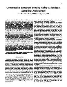
RELEVANCE BPS is used in many fields [2]: communications, optics, radar, sonar, measurement, instrumentation, and more recently, all kinds of wireless devices and software defined radio [6], [7]. In any discipline, increasing technological complexity makes conceptual simplification of the basic principles ever more crucial. For BPS, this includes simpler derivations of safe rules for the sampling rates. PREREQUISITES To understand the approach, high school geometry suffices, provided one accepts on faith the reasoning leading to spectral replication (Figure 1). This reasoning itself assumes some basics of signal processing. PROBLEM STATEMENT AND OBJECTIVES As explained later, the result of sampling can be modeled by spectral replication, periodic in the frequency domain. This is visualized for baseband sampling in Figure 1 and for BPS in Figure 2. The issue is then avoiding aliasing, that is, overlap between replicas, which results in their addition (summation) and thereby makes reconstruction of the original signal more difficult (requiring special signal properties and methods).

Digital Object Identifier 10.1109/MSP.2012.2192969 Date of publication: 12 June 2012

Why typical derivations of the conditions are considered tricky [1], [2] may be explained by two major flaws: 1) they use loose verbal arguments instead of mathematical methods 2) they are based on snapshots of replicas for separate sampling rates (as in Figure 3), which cannot convey the continuous way in which replicas shift with the sampling rate. Such arguments literally and figuratively have gaps and are prone to oversight. Which results are trustworthy requires corroboration by methods that are both simpler and more rigorous by the common standards of engineering mathematics. Of course, existing derivations may satisfy specialists who can fall back on some deeper insight that is not easy to articulate or reflect in the arguments. Still, the novice as well as the diligent reader is left with the urge to (re)do things differently, requiring only general deductive abilities rather than hindsight. In fact, the author devised the described approach for his own initial understanding of BPS, forewarned by [1]. Although we also give a taste of a formal derivation, in the geometric version the order of derivation is the opposite from the usual. In the literature [1], [2] one starts by deriving inequalities of the form

A

A

−3s

−2s

−s

−B 0 +B (a)

+s

+2s

+3s

f

−4s −3s

−2s

−s

0 (b)

+s

+2s +3s +4s

f

[FIG1] Spectral replication in baseband sampling (a) spectral replication for s , 2B and (b) overlapping replicas (aliasing) for s , 2B.

IEEE SIGNAL PROCESSING MAGAZINE [90] JULY 2012

1053-5888/12/$31.00©2012IEEE

2fu 2fL or # fs # n n21 2fc 1 B 2fc 2 B # fs # m11 m

A

−s

s

(1)

(for proper n, m) where fu is the upper, fL the lower and fc the center frequency, and B is the bandwidth. From the formulas, diagrams similar to Figure 4 follow [1, Figs. 2–11], [2, Fig. 4], [3, Fig. 3.4]. The geometric approach first yields the diagrams, and the formulas follow by inspection. Also, to avoid notational clutter in formulas and figures, simple, direct symbols like s, L are used instead of subscripting as in fs, fL. The organization is as follows. After a reminder of basic sampling concepts, a brief intermezzo discusses the formal derivation of sampling conditions for BPS. The geometric recast first derives the basic diagram for bandpass sampling and then shows how to extract properties of interest by mere inspection. The geometry of aliasing yields sampling conditions as formulas and as the usual normalized sampling diagram. Zooming in on crowding regions yields the geometry of the bandpass Nyquist rate. Finally, conditions to preserve spectral direction are extracted. Further examples show how to approach similar problems geometrically. To the geometrically inclined, the diagrams are self-explanatory as “proofs without words” [8], and further text could be skipped at various points. Still, as geometry seems an “endangered art,” some readers will better appreciate the generality of the approach by some comments in words. BACKGROUND To make this note self-contained, we summarize a few basic results, also found in most textbooks [1], [4]. Sampling a continuous-time (CT) signal x periodically with interval T or rate s J 1/T(s . 0) means deriving a sequence x T with x T 1 n 2 5 x 1 nT 2 for integer n. As outlined in [4], the inconsistent notation x 3 n 4 is avoided. The question is: to what extent can the CT

−C − s C − 3s

−C C − 2s

−C + s C−s

–C + 3s f C+s

–C + 2s C

[FIG2] Spectral replication by BPS: structure.

s = 32 −62

−34 −30

−2 2 (a)

30 34

f (MHz)

62

s = 25 −55

−45

−30

−20

−5

(b)

5

20

30

45

55

s = 18 −60

−48 −42

−30 −24

−12 −6

6 12

24 30

42 48

60

(c) s = 11

−58

−47

−36

−25

−14

−3 0 (d)

8

19

30

41

52

63

[FIG3] Examples of spectral replication by BPS.

signal x be reconstructed from the sequence xT ? To model sampling, one usually represents x T by a CT signal x^ T in which each sample x 1 nT 2 is attached to a delta function at nT. Using d 11 t2nT 2 /T 2 rather than d 1 t 2 nT 2 supports sanity checking by dimensionality

(2)

n52`

The Fourier transform F x^ T of x^ T can directly be calculated termwise 1 F x^ T 2 1 v 2 `

`

n52` `

2`

5 a x 1 nT 2 3 d 1 t/T2n 2 e2jvt dt 5 T a x 1 nT 2 e 2jv nT .

n52`

5 1x2t where

(3)

n52`

Visualizing and interpreting the spectrum is easier by calculating F x^ T in a different way, a technique known as the Fubini principle [9]. To this effect, (2) is rewritten using the sifting property of d


`

1 t/T 2 ,

1u2 5 a d1u 2 n2.

(4)

n52`

Now is periodic, and by Fourier series ` expansion 1 t/T 2 5 g k52` e jkVt where V 5 2p/T. Hence, `

`

x^ T 1 t 2 5 a x 1 nT 2 d 1 t/T2n 2 .

`

x^ T 1 t 2 5 a x 1 t 2 d 1 t/T2n2

`

1 Fx^ T 2 1 v 2 5 3 x 1 t 2 a e jkVte2jvtdt 2` `

k52`

5 a 1 Fx 2 1 v2kV 2 .

(5)

k52`

This shows that the spectrum F x of the original signal x is replicated in F x^ T infinitely often and V apart. For baseband sampling, the spectrum is assumed zero for frequencies f 1 5v/2p 22 outside some interval 3 0, B 4 (hence, also 3 2B, 0 4 ), where B is the bandwidth. The spectrum resulting from sampling with rate s is visualized in Figure 1. For sampling rates 2B and below, the replicas overlap [Figure 1(b)], and

[lecture NOTES]

continued

Recovering the given signal from samples is “hard” if replicas overlap (aliasing). As the sampling rate s varies (conceptually), replicas move in different directions “through” each other in a manner commonly visualized by redrawing Figure 2 for various s. Figure 3 illustrates this for C 5 30 MHz, B 5 6 MHz, and s 5 11 MHz, 18 MHz, 25 MHz, and 32 MHz. Typical reasoning and formulas are based on analyzing limiting cases (abutment of spectra), but interpretation of such a fragmented view is tricky and prone to oversights. More complete views are offered by systematic derivations, e.g., formally or geometrically.

s/2B 6

O=1

m=0 5 (Q + 1)/O (Q:= L/B )

m=1

4

O=2

Q /O

3

m=2

2

O=3 m=3 O=4 O=5

1 L/B

0 0

1

2

3

4

5

6

7 Q

[FIG4] Normalized sampling rates.

(5) sums them. Since two terms cannot be determined from their sum, overlaps make reconstructing x more difficult. This situation is called aliasing because components of the spectrum can be seen as “masquerading” for others. If the sampling rate s is strictly greater than 2B, no aliasing occurs [Figure 1(a)], and x can be reconstructed from F x^ T by extracting the part from 2s/2 to s/2 when calculating the inverse transform using (3) V/2

x1t2 5

1 1 F x^ T 2 1 v 2 dv 2p 32V/2 V/2

` T 2jvnT jvt 5 a x 1 nT 2 e e dv 3 2p n52` 2V/2

hence, `

x 1 t 2 5 a x 1 nT 2 sinc 1 t/T 2 n 2 , n5 2`

where

A

–U –L –C

L

C

U

f

[FIG5] Bandlimited signal and symbol conventions.

sinc u5 if u5 0 then 1 else 1 sinpu/pu 2 . (6) Here s . 2B was a sufficient condition. For the simple reconstruction (6) to hold, it is also necessary: if x 1 t 2 5 cos 1 V/2 2 a 2 t and xr 1 t 2 5 cos 1 V/2 1 a 2 t then x 1 nT 2 5 cos np cos naT 5 xr 1 nT 2 . Taking x 1 t 2 5 A cos 1 Vt/22w 2 is also instructive. Necessity for (6) does not imply necessity for other schemes. A signal is bandlimited if its spectrum is zero outside an interval 3 L, U 4 (and hence also 3 2U, 2L 4 2 , called the support. Figure 5 shows the symbol conventions. The bandwith is B J U 2 L and the center frequency is C J 1 L 1 U 2 /2. For the discrete mathematics aspects considered here, all one needs to remember about the sampling model is that a component in the original signal spectrum at an arbitrary frequency, say f, is replicated at f, f 6 s, f 6 2s, f 6 3s, etc.; in brief: f 1 ks for k in Z (the integers). An example: sampling at s 5 25 MHz yields for f 5 30 MHz replicas at 30 MHz, at 55, 80, 105, cMHz and at 5,220,245, cMHz. Spectra resulting from sampling a bandlimited signal for given C and s are typically visualized as in Figure 2, including also the replicas of the part centered at 2C.


INTERMEZZO: ON THE FORMAL DERIVATION OF PROPER SAMPLING RATES FOR BPS Given the replication model as described, overlap occurs if and only if replicas of the form f 1 ks and c 1 js coincide for some f in 3 L, U 4 , c in 3 2U,2L 4 and integer values of k and j. Formally, E f : 3 L, U 4 . E c : 3 2U, 2L 4 . E k : Z. E j : Z # f 1 ks 5 c 1 js.

(7)

One can read E v : V # P 1 v 2 in words as “there exists a (value) v in (set) V such that P 1 v 2 .” Functional predicate calculus [5] allows simplifying (7) step-bystep by chaining equalities in the style engineers routinely use and appreciate in calculus. This is illustrated in Figure S1 in “A Taste of Formal Predicate Calculus in Deriving BPS Conditions.” Here is an informal summary, which arguably provides a more direct insight than most derivations of BPS rates in the literature. If overlap occurs, f 1 ks 5 c 1 js or, equivalently, f 2 c 5 1 j 2 k 2 s 5 ,s for some integer ,. Since f 2 c [ 3 2L, 2U 4 , this implies ,s [ 3 2L, 2U 4 or, equivalently, 2L # ,s # 2U for some integer ,. Conversely, if 2L # ,s # 2U for some integer ,, then ,s/2 [ 3 L, U 4 . Choosing f 5 ,s/2 and c 5 2,s/2 yields f 1 ks 5 c 1 js for any integer k and j that satisfy j 2 k 5 ,. This reflects overlap.

A TASTE OF FORMAL PREDICATE CALCULUS IN DERIVING BPS CONDITIONS For BPS, the danger of aliasing (overlap) at sampling rate s (without loss of generality, s . 0) is expressed as A 1 s 2 , where A is a predicate defined as follows, up to omitted terms that do not change the end result.

A (s )

[L, U ] [L, U ] [L, U ]

Definition Arithmetic

[–U, –L ] k [–U, –L ] k [–U, –L ] [L, U ] [–U, –L ] [L, U ] [–U, –L ] [L, U ] [–U, –L ]

Change var. Lemma A Leibniz Swap Distrib.

A 1 s 2 ; E f : 3 L, U 4 . E c : 3 2U,2L 4 . E k : Z. E j : (S1) Z # f 1 ks 5 c 1 js.

2L 2L 2L 2L

Arithmetic One-pt. rule

s

2U

s s s

2U 2U

[L, U ] [L, U ] [L, U ]

ks

j j

js ( j – k)s

s s 2L s 2L s 2L [–U, –L ]

2U 2U

s s

2U s s

[–U, –L ] s [–U, –L ]

2U Lemma B This can be simplified step-by-step by U –U –L 2L 2U (properties ) Lemma A L chaining equalities, which is the style [–U, –L ] Proof take [2L, 2U] /2 [L, U ] Lemma B engineers routinely use and appreciate in calculus. Here, obviously the calculation rules are those of predi- [FIGS1] Example of a calculational derivation of aliasing conditions. cate calculus [5]. Such a calculation is illustrated in Figure S1, only to convey the flavor, as full also similar to multiple integrals awaiting their turn for understanding by the uninitiated may require careful simplification. study. The roles of variables and bindings in Ev : 3 a, b 4 # P 1 v 2 Most importantly: necessity and sufficiency are handled and in eab f 1 v 2 dv are similar. Multiple quantifiers ( E, 4) are together by logical equality ( ; ).

Hence, E , : Z # 2L # ,s # 2U is both necessary and sufficient for overlap, indicating “forbidden” rates. A convenient normalized form is E , : Z # Q # ,s/2B # Q 1 1 where Q J L/B, visualized in Figure 4. BANDPASS SAMPLING GEOMETRY As an alternative to formal logic, geometric loci provide a complete picture of the continuous shift in function of s.

k = −3 j = −1

s

k = −1

j=0

k = −2

−φ + s

−φ

j=1

k=0

j=2

φ−s

φ − 2s

φ − 3s

cally as an s-coordinate, covering varying sampling rates in a continuous and manifestly complete way. The replicas of a component f are found at frequencies f satisfying f 5 f 1 ks for k : Z. The equation f 5 f 1 ks for f as a function of s is a straight line for each k; similarly f 5 2f 1 js for each j. This yields two line bundles, as shown in Figure 6. Given s, the replicas of 6f are at the intersections of these bundles with the

The idea is so simple that geometryminded or even just graphical-minded people can skip the text and infer everything from only Figures 5–9. Still, some additional explanations and examples are given. The vertical dimension in diagrams (such as Figure 2) is used for mere token shapes that cause visual clutter with little useful information: only the frequency intervals matter. This dimension will be put to better use, specifi-

φ+s −φ + 2s

φ

−φ + 3s

j=3 k=1

k = −4

j=4

j = −2

k=2

j = −3 j = −4

k=3 k=4 −φ

0

[FIG6] Geometry of frequency replication; indexing.


φ

f

[lecture NOTES]

continued

s

U1

(Sampling Rate)

2U O=1 2L L1

j=0

j=1

k = –1

k=0

U1′ U2

2U/2

O=2 2L/2 L1′

Example

k = –2

L2 j=2 U3

Typical Parallellograms k = –3

Hatched for O = 3 Only U2′

O=3 j=3

2U/3 2L/3

L3

U4

2U/4 2L/4

O=4 L4

L2′

F

D −U −L

M

E 0

G L

U

f

[FIG7] BSG diagram.

horizontal at s, as illustrated by the dotted line. This line is drawn for the arbitrarily chosen proportion s/f 5 5/6, so a numeric example is f 5 30 MHz and s 5 25 MHz. Another example: assuming f fixed at 30 MHz and lowering the dotted line to let s decrease from 25 MHz, Figure 6 shows that the firsttime replicas of 6f coincide is at the intersections of the line pairs with j 2 k 5 3 (e.g., k 5 21 and j 5 2), yielding s 5 20 MHz. Imagining f to be the center frequency of some bandlimited signal (with B 2 0), clearly the replicas of the

edges of the spectra collide sooner than those of their center frequencies, as analyzed next. In the sampling model, all signal components in 3 L, U 4 are replicated as explained, yielding replicas with support 3 L 1 ks, U 1 ks 4 for k : Z. For instance, assuming s 5 25 MHz and with all data in MHz, replicas of 3 27, 33 4 are 3 27, 33 4 itself, 3 52, 58 4 , 3 77, 83 4 , c and 3 2, 8 4 , 3 223, 217 4 , c. For the negative frequencies, 2f has replicas 2f 1 js for j : Z a n d 3 2U, 2L 4 h a s r e p l i c a s 3 2U 1 js, 2L 1 js 4 f o r j : Z. F o r instance, replicas of 3 233, 227 4 are


3 233, 227 4 itself, 3 28, 22 4 , 3 17, 23 4 , c a n d 3 258, 252 4 , 3 283, 277 4 , c. A simple way to represent this geometrically for continuously variable s is marking the endpoints of the supports by a line bundle pair at 6L and one at 6U, forming beams. This yields the bandpass sampling geometry (BSG) diagram of Figure 7. For example, in drawing Figure 7, we chose U/L 5 10/9, so we can take L 5 18 MHz, U 5 20 MHz. With this scale, the line marked “example” is at s 5 16 MHz and the thick segments represent support replicas.

EXTRACTING PROPERTIES BY GEOMETRY Overlaps between spectra are apparent in Figure 7 as the parallellogram-shaped beam intersections. The corresponding s-regions are shaded in red. The diagram suggests that it is more direct to characterize the forbidden regions rather than their complement, the allowed intervals, as in the inequalities (1) using a parameter m or n. Of course, (1) then also follows directly, as noted below. For indexing the forbidden regions, a convenient parameter is , J j 2 k because parallellograms with equal ,value (as hatched for , 5 3 in Figure 7) have the same projection on the s-axis. Overlaps for k 5 0 (, 5 j) are representative for all those with the same ,-value, without risking oversights. With the points labeled as in Figure 7, the sampling rate in forbidden region , is seen by inspection to satisfy EL, # s # GU, (shown for , : 1..4). By g e o m e t r y , EL, 5 DE/, 5 2L/, a n d GU, 5 FG/,5 2U/,. Hence, the forbidden s-values are given by 2L 2U #s# for any positive integer ,. , , (8) Noting that each forbidden region in Figure 7 has its own ,-value, the allowed regions in between are characterized by two consecutive ,-values, which directly yields the inequalities (1) with some name changes. By geometry, without (8), we derive an equivalent but more direct diagram for the sampling conditions. In Figure 7, the values EL, (for 2L/,) and GU, (for 2U/,) delimiting the regions are read along different vertical lines, which is inconvenient. However, DE and FG have common midpoint M. Hence, from DM 5 DE/2 it follows that MLr, 5 EL , /2. Similarly, from FM 5 FG/2 it follows that MUr, 5 GU, /2. Hence, the desired values EL, and GU, can be read at half the scale as MLr, and MUr, along the same vertical at M, where also the varying s-values read along the verticals at E and G are projected as s/2. To turn Figure 7 into a diagram where usable sampling rates can be

read conveniently, note that DM 5 L, and move the origin to D. Now, as L varies, the j-beams do not change (the k-beams were already obviated). Their

CONCEIVABLY, ALIASING MIGHT BE RESOLVABLE EVEN IF REPLICAS OVERLAP, PROVIDED THE SAMPLED SIGNAL SATISFIES CERTAIN PROPERTIES. intersections Lr, and Ur, with the (now variable) vertical at M always show the region boundaries 2L/, and 2U/, at half the scale ( s/2). Hence, the j-beams form a diagram indicating forbidden sampling rates. This diagram is normalized by dividing all frequencies by B, yielding Figure 4. Clearly the very lowest rate is 2B, and requires integer L/B; in fact, L/B 5 ,. The vertical above the dot covers baseband sampling. A pictorially identical diagram is also found in [1]–[3], but here we derived it “on sight” by geometry without any calculation or even construction lines. The labeling of the axes is usually slightly different (R J U/B instead of Q J L/B, and s/B instead of s/2B). For easy comparison, Figure 4 is complemented by showing the m-values used in [1] to index the acceptable regions and in the rightmost inequality in (1). Figure 7 suggests something interesting at low sampling rates. Indeed, the BSG shows alternating allowed and forbidden regions. As , increases, regions crowd together (not drawn, but shaded in grey). The allowed regions become

narrow faster than the forbidden ones, which overlap at some stage. Overlap starts when the lower bound EL, of region , ceases to be greater than the upper bound GU,11 of region , 1 1. Calculation is simple (2U/ 1 , 1 1 2 = 2 L/,52 1 U 2L 2 / 1 ,112, 2 52B 2 , but geometry visualizes what is going on. Figure 8 zooms in on the situation where EL, 5 GU,11. This does not necessarily occur for whole values of ,, but fractional values do not affect the essence. Let K be the intersection between DL, and FU,11. Then ^ DKF and ^ L,KU,11 are congruent, so the projection of K on FG is the midpoint M. M o r e o v e r , MK 5 FM/ 1 ,11 2 5 DM/,51 FM2DM 2 / 1 ,112,2 5B. Hence EL, 5 GU,11 5 2B. This is the bandpass Nyquist rate, consistent with Figure 4. Note: , 5 L/B. Thus far, we considered supports, ignoring spectrum inversion (or reversal) [1]. Inverted replica stem from the negative frequencies. Usually, this is symbolized by a sloped line in the token amplitude diagram (Figure 2). Here we attach direction to supports by vectors: a left to right vector for beams coming from positive frequencies, and an inverse vector for beams from negative frequencies. In the BSG, direction is immediately clear, and vectors need not be drawn. Yet, for illustration, vectors at various sampling rates are shown in Figure 8, a “zoomed in” part of Figure 7. For some spectra, such as those resulting from single sideband modulation, one may want sampling rates yielding noninverted replicas next to the origin [1]. Figure 7 shows that replicas near the origin require even ,,

2U UO

2L

O LO

UO+1 O+1

K B F

D

M

[FIG8] BSG: crowding region.


E

G

[lecture NOTES]

continued

O = 2i s = 2L/O

[FIG9] Spectral inversion.

p/F p p/ F

Geometry helps disentangling this spiderweb. Observe that bundling occurs for f/F 5 0 at p/F 5 N. Letting k J n 1 N y i e l d s p/F 5 1 k 2 n 2 1 nf/F, resulting in bundling for f/F 5 1 at p/F 5 k. By analogy with Figure 6, where intersections are periodic on a horizontal, in Figure 10 they are periodic on a vertical. So it suffices to consider just the rational values of f/F (which a posteriori is seen from the formulas). This simplifying observation was also made in [12].

2.0 1.5 1.0 0.5 0

fF f/ f/F 0

0.5

WHAT WE HAVE LEARNED To study frequency-related signal processing issues, geometry is an attractive alternative to loose arguments and case analysis. Advantages are clarity, intuitive appeal, simplicity, and reliability (no danger of oversights), proving once again that “a picture is worth a thousand words” [8].

1.0

[FIG10] Geometry of intermodulation products.

and Figure 9 shows that, for noninversion, s 5 L/i for positive integer i. This is equivalent to the formula fso 5 1 2fc2B 2 /meven in [1]. FURTHER RAMIFICATIONS Conceivably, aliasing might be resolvable even if replicas overlap, provided the sampled signal satisfies certain properties. In such cases, the model must be more detailed, with geometry in three dimensions (amplitude in function of f and s). A recent paper [10] uses a diagram, traceable back to [11], to determine cross products. It contains “rays” as in Figure 6. Cross products resulting from, say, 1 A cos 2pFt 1 a cos 2pft 2 j have frequencies given by p 5 NF 1 nf for N and n in Z. The resulting diagram for f # F is shown in Figure 10. Some cross products are wanted (e.g., for mixing), most are not. Unwanted products are avoided by selecting f/F away from undesirable intersections.

GEOMETRY OFTEN PROVIDES SIMPLER EXPLANATIONS AND HENCE BETTER INSIGHT FOR STUDENTS AND PROFESSIONALS. Whereas “a formula is worth a thousand pictures” [13], the implied proviso is that the derivation is by formal symbolic calculation, not loose word arguments. This can be done clearly and succinctly for BPS by functional predicate calculus [5], but since the required basis is not as generally available as geometry, here we chose geometry. Yet, the observations by Lee and Varaiya [4] suggest that, in the long run, predicate calculus may be as important to digital signal processing engineers as differential and integral calculus. Finally, geometry often provides simpler explanations and hence better insight for students and professionals. We see it as complementing, not replacing, other methods, since diversity of views deepens understanding more than a single isolated approach.


Just for the sake of completeness, we mention that sampling at lower rates than considered in the ShannonNyquist model is possible for signals with certain compressibility characteristics [14]. This is an entirely different issue not discussed here. AUTHOR Raymond Boute (Raymond.Boute@ pandora.be) is emeritus professor at the Faculty of Engineering Sciences, Department of Information Tecchnology (INTEC), Ghent University (Belgium). His research interests are in unifying mathematical modeling in classical and computer engineering. REFERENCES

[1] R. G. Lyons, Understanding Digital Signal Processing. Englewood Cliffs, NJ: Prentice-Hall, 2004. [2] R. G. Vaughan, N. L. Scott, and D. R. White, “The theory of bandpass sampling,” IEEE Trans. Signal Processing, vol. 39, no. 9, pp. 1973–1984, Sept. 1991. [3] Y. Sun, “Generalized bandpass sampling receivers for software defined radio,” Ph.D. dissertation, Roy. Inst. Technol., Sweden, May 2006. [4] E. A. Lee and P. Varaiya, Structure and Interpretation of Signals and Systems. Reading, MA: Addison-Wesley, 2003. [5] R. Boute, “Functional declarative language design and predicate calculus, a practical approach,” ACM Trans. Program. Lang. Syst., vol. 27, no. 5, pp. 988–1047, Sept. 2005. [6] A. Mahajan, M. Agarwal, and A. K. Chaturvedi, “A novel method for down-conversion of multiple bandpass signals,” IEEE Trans. Wirel. Commun., vol. 5, no. 2, pp. 427–434, Feb. 2006. [7] Y. Sun and S. Signell, “Implementation aspects of generalized bandpass sampling,” in Proc. 15th European Signal Processing Conf. (EUSIPCO 2007), M. Doman´ski, R. Stasin´ski, and M. Bartkowiak, Eds. 2007, pp. 1975–1979. [8] R. B. Nelsen, Proofs Without Words II. Washington, DC: The Mathematical Association of America, 2001. [9] K. Penev, “The Fubini principle,” Amer. Math. Monthly, vol. 115, no. 3, pp. 245–248, Mar. 2008. [10] C. Drentea, “The Star-10 transceiver,” QEX, no. 245, pp. 3–17, Nov./Dec. 2007. [11] T. T. Brown, “Mixer harmonic chart,” Electronics, vol. 24, pp. 132–134, Apr. 1951. [12] H. Rutgers. (1995). Choosing frequencies in heterodynes [Online]. Available: http://www.byrutgers.nl/PDFiles/Frequencies in Hetrodynes.pdf [13] E. W. Dijkstra, “A formula is worth a thousand pictures,” in Millennial Perspectives in Computer Science(Proc. 1999 Oxford-Mic rosoft Symp. in Honour of Sir Tony Hoare), J. Davies. B. Roscoe, and J. Woodock, Eds. Basingstoke UK: Palgrave, 2000, pp. 99–107. [14] E. J. Candès and M. B. Wakin, “An introduction to compressive sampling,” IEEE Signal Processing Mag., vol. 25, no. 2, pp. 21–30, Mar. 2008.

[SP]