The Global Crop Water Model (GCWM): Documentation and first ...

07 The Global Crop Water Model (GCWM): Documentation and first results for irrigated crops.

RESEARCH REPORT Stefan Siebert

•

Petra Döll

March 2008

Frankfurt Hydrology Paper

The Global Crop Water Model (GCWM): Documentation and first results for irrigated crops

Research report

Stefan Siebert and Petra Döll

Institute of Physical Geography University of Frankfurt (Main)

March 2008

Frankfurt Hydrology Papers: 01 02 03 04 05 06 07

A Digital Global Map of Irrigated Areas – An Update for Asia Global-Scale Modeling of Nitrogen Balances at the Soil Surface Global-Scale Estimation of Diffuse Groundwater Recharge A Digital Global Map of Artificially Drained Agricultural Areas Irrigation in Africa, Europe and Latin America - Update of the Digital Global Map of Irrigation Areas to Version 4 Global data set of monthly growing areas of 26 irrigated crops The Global Crop Water Model (GCWM): Documentation and first results for irrigated crops

Institute of Physical Geography, Frankfurt University P.O. Box 11 19 32, D-60054 Frankfurt am Main, Germany Phone +49 (0)69 798 40220, Fax +49 (0)69 798 40347 http://www.geo.uni-frankfurt.de/ipg/ag/dl/index.html

Please cite as: Siebert, S. & Döll, P. (2008): The Global Crop Water Model (GCWM): Documentation and first results for irrigated crops. Frankfurt Hydrology Paper 07, Institute of Physical Geography, University of Frankfurt, Frankfurt am Main, Germany

The Global Crop Water Model (GCWM) – Abstract

4

Abstract A new global crop water model was developed to compute blue (irrigation) water requirements and crop evapotranspiration from green (precipitation) water at a spatial resolution of 5 arc minutes by 5 arc minutes for 26 different crop classes. The model is based on soil water balances performed for each crop and each grid cell. For the first time a new global data set was applied consisting of monthly growing areas of irrigated crops and related cropping calendars. Crop water use was computed for irrigated land and the period 1998 – 2002. In this documentation report the data sets used as model input and methods used in the model calculations are described, followed by a presentation of the first results for blue and green water use at the global scale, for countries and specific crops. Additionally the simulated seasonal distribution of water use on irrigated land is presented. The computed model results are compared to census based statistical information on irrigation water use and to results of another crop water model developed at FAO.

The Global Crop Water Model (GCWM) – Contents

5

Table of Contents 1

Introduction ....................................................................................................................... 6

2

Data and methods.............................................................................................................. 7 2.1

Cropping pattern and cropping season.............................................................................. 8

2.2

Climate input...................................................................................................................... 11

2.3

Reference evapotranspiration (ET0)................................................................................. 13

2.4

Maximum crop evapotranspiration (ETc)........................................................................ 16

2.5

Soil water balances performed to compute actual evapotranspiration (ETa)............... 17

2.6

Crop water use ................................................................................................................... 18

2.7

Evapotranspiration on days with snow covered or frozen soil ...................................... 18

2.8

Application of the model for irrigated crops and the period 1998 – 2002 .................... 19

3

Results.............................................................................................................................. 19

4

Discussion........................................................................................................................ 24 4.1 Comparison of the simulated irrigation water requirements to census-based statistical information ..................................................................................................................... 24 4.2 Comparison of the simulated irrigation water requirements to agricultural water use and irrigation water requirement reported by FAO for 90 developing countries .................... 27

5

Summary and conclusions .............................................................................................. 28

References................................................................................................................................ 30 Annex A – Tables Annex B - Figures

The Global Crop Water Model (GCWM) – Introduction

1

6

INTRODUCTION

Knowledge about where on earth irrigation occurs and how much water is used for this purpose is an important basis for understanding the role of agriculture for food security or the relevance of agriculture for sustainable water management. About 279 Mha of agricultural land were equipped for irrigation around the year 2000 (Siebert et al., 2006). It was estimated that about 2700 km3 yr-1 of fresh water is withdrawn from surface water bodies or aquifers to irrigate crops which represents about 70% of the global water withdrawals for agriculture, households and industry (FAO, 2007; Shiklomanov, 2000). Parts of the freshwater withdrawals are return flows that could potentially be reused downstream. The difference between irrigation withdrawal water use (IWWU) and return flows, the so called irrigation consumptive water use (ICWU), was estimated at 1752 km3 yr-1 for the year 2000 (Shiklomanov, 2000) which represents more than 90% of the total consumptive water uses in all sectors. To support sustainable water management, water use is usually compared to available water resources. This allows to compute indicators for water scarcity, sustainability of water resources use or dependency on external resources (e.g. FAO, 2007; Lehner et al., 2006; Alcamo et al., 2003a; Vörösmarty et al., 2000; Seckler et al., 2000; Alcamo et al., 1997). One of the models applied to simulate water resources and water use at the global scale is the WaterGAP model (Alcamo et al., 2003b). The model uses daily time steps on a resolution of 30 arc minutes. It calculates runoff and river discharge as well as water use for irrigation, livestock, manufacturing, cooling of power plants, domestic households and livestock on the other hand. The Global Irrigation Model (GIM), which is the irrigation sub model of WaterGAP, simulates the cropping pattern, cropping intensity and the related irrigation water requirement for rice and the group of non-rice crops (Döll and Siebert, 2002). The model requirements for statistical input data are relatively low to facilitate the model use for analyses of global change scenarios. Using the most recent version 4 of the Digital Global Map of Irrigation Areas (Siebert et al., 2006) as a model input, the global net irrigation water requirement, which is the amount of water needed to ensure optimal growth of irrigated crops, was computed at 1322 km3 yr-1 for the period 1998 – 2002. The gross irrigation water requirement, which is the water withdrawal from surface or ground water resources assuming optimal growing conditions and specified irrigation efficiencies, was computed at 3008 km3 yr-1 (Siebert, unpublished). The inventories of water resources and water uses as mentioned before do not include the so-called virtual water flows (Allan, 1993). Virtual water content of a commodity is defined as the volume of water required to produce the specific commodity. Virtual water flows are induced by trade. If a specific good is imported by country A and exported by country B then the virtual water content of the specific good is also transported from country B to country A and thus a virtual water flow appears from country B to country A. The practical importance of those virtual water flows is that countries poor in water resources can participate in water resources located in water rich countries by importing goods produced in those countries instead of using their own water resources to produce these goods. A water saving can also appear at the global scale namely if the amount of water needed to produce a

The Global Crop Water Model (GCWM) – Introduction

7

commodity in the exporting country is lower than the amount of water that would be needed to produce the commodity in the importing country (Oki and Kanae, 2004). In the history, virtual water trade between nations was negligible, in particular for agricultural products, because only very minor portions of food were traded over long distances. But nowadays, in the era of globalization and the related tremendous increase in international trade, virtual water trade is being discussed as an effective instrument to reduce water scarcity and food insecurity (Yang et al, 2006). Therefore, future inventories of water balances for nations or watersheds should also include virtual water flows. It is necessary to distinguish blue and green virtual water flows. Blue water is withdrawn from surface water bodies or ground water while green water is provided by precipitation. The relevancy of both types of virtual water is different. For example, there is competition of the different water use sectors for blue water only. First estimates quantify the global volume of virtual water flows related to international trade at 1625 km3 yr-1. About 80% of these virtual water flows relate to the trade in agricultural products, while the remainder is related to industrial product trade (Chapagain and Hoekstra, 2004). Water saving at the global scale by virtual water trade was estimated at 450 km3 yr-1 (Oki and Kanae, 2004), 352 km3 yr-1 (Chapagain et al., 2006) or 337 km3 yr-1 (Yang et al., 2006). However, the uncertainties in the estimates are still very large. Crop water use, for example, was computed in these studies based on climate values averaged for each country. Additionally, blue and green water flows are not given separately which makes it difficult to interpret the specific meaning of the results. In this study we make a first step towards improving estimates of blue and green virtual water content by presenting a crop water model that simulates requirements of blue and green water for 23 major crops and 3 crop groups in daily time steps. The spatial resolution of the Global Crop Water Model (GCWM) is 5 arc minutes by 5 arc minutes. The final modeling results will be made available to the public via the web site of the virtual water fluxes project at the University of Frankfurt (Main) at http://www.geo.unifrankfurt.de/ipg/ag/dl/forschung/Virtual_water/index.html. In section 2 of this paper we describe the methodology used to develop the model and the input data necessary to use the model. First results for irrigated crops are presented in section 3. In section 4 we compare our results to those of other models and we also discuss limitations and major sources of uncertainties. In section 5 we finally give a summary and draw conclusions.

2

DATA AND METHODS

In this section we describe the input data used by the new model and the methodology to compute crop water uses. The main differences of the new Global Crop Water Model compared to the already existing Global Irrigation Model of WaterGAP are that the cropping pattern and cropping calendar are required as input data set, that the number of crops increased from 2 to 26, that water requirements for irrigated agriculture and water use for rainfed agriculture are computed based on the same methodology which requires also a

The Global Crop Water Model (GCWM) – Data and methods

8

TABLE 1 Differences in methodology and input data requirements between the new Global Crop Water Model (GCWM) and the most recent version 2.1f of the WaterGAP model GCWM

WaterGAP 2.1f

Blue (irrigation) water requirement of crops

Computed in GCWM based on a soil water balance

Computed in GIM, the irrigation model of WaterGAP (Döll and Siebert, 2002) as the difference between potential evapotranspiration and effective precipitation

Green (precipitation) water use of crops

Computed in GCWM based on a soil water balance

Computed in WGHM, the hydrology model of WaterGAP (Döll et al., 2003) based on a soil water balance

Number of crop classes

26

1 for rainfed agriculture and 2 (rice, nonrice) for irrigated agriculture

Cropping pattern and cropping season

Input from file

Simulated by the models

Method to compute reference evapotranspiration

Penman-Monteith or PriestleyTaylor

Priestley-Taylor

Spatial resolution

5 arc minutes, results can be aggregated to 30 arc minutes

30 arc minutes

calculation of the actual evapotranspiration, that the modeling of water requirements is based on a soil water balance, that two different methods are implemented to compute reference evapotranspiration and that the spatial resolution of the model changed from 30 to 5 arc minutes (Table 1). 2.1 Cropping pattern and cropping season The data set used to define the cropping pattern and the growing seasons for the 26 crop classes listed in Table 2 is documented in Portmann et al. (2008). The data set refers to the situation around the year 2000 and consists of two parts: monthly grids of growing areas for each of the crop classes with a spatial resolution of 5 arc minutes by 5 arc minutes and a list of cropping calendars for 402 spatial units like countries, federal states, provinces (Figure 1) consistent to the grids of monthly growing areas. The data set explicitly considers multicropping practices. By now, it is available for irrigated crops only but data for the related rainfed crops will become available soon. The list of cropping calendars (for an extract see Figure 2) provides for each crop class and up to five sub-crops the growing area, the month when the growing season starts and the month when the growing season ends. As an example we describe in the following the cropping calendar for the unit California (Figure 2). California has the unit number 840005 that appears in the first column. The crop number is given in the second column and the number of sub-crops in the third column. Beginning with the fourth column total growing area, first month of growing season and last month of growing season are listed for each subcrop. Thus, the second line can be interpreted as follows: In unit 840005 (California) there are two sub-crops of crop 1 (wheat). The first sub-crop is growing on 98723.06 ha in the period September – June and the second sub-crop is growing on 38363.79 ha in the period April to August. Here the first sub-crop could be irrigated winter wheat while the second sub-crop will be irrigated spring wheat. For the crops sugar cane (12), oil palm (14), citrus (18), date palm (19), grapes (20), cocoa (22), coffee (23), others / perennial (24) and managed grassland / pasture (25) the first month of the growing season will be always January (1) and the last

Wheat (1) Maize (2) Rice (3) Barley (4) Rye (5) Millet (6) Sorghum (7) Soybeans (8) Sunflower (9) Potatoes (10) Cassava (11) Sugar cane (12) Sugar beets (13) Oil palm (14) Rapeseed / canola (15) Groundnuts / Peanuts (16) Pulses (17) Citrus (18) Date palm (19) Grapes / vine (20) Cotton (21) Cocoa (22) Coffee (23) Others (perennial) (24) Managed grassland/pasture (25) Others (annual) (26)

0.15 0.17 0.17 0.15 0.10 0.14 0.15 0.15 0.19 0.20 0.10 0.00 0.20 0.00 0.30 0.22 0.18 0.00 0.00 0.30 0.17 0.00 0.00 0.00 0.00 0.15 0.25 0.28 0.18 0.25 0.60 0.22 0.28 0.20 0.27 0.25 0.20 0.00 0.25 0.00 0.25 0.28 0.27 0.00 0.00 0.14 0.33 0.00 0.00 0.00 0.00 0.25

0.40 0.33 0.44 0.40 0.20 0.40 0.33 0.45 0.35 0.35 0.43 1.00 0.35 1.00 0.30 0.30 0.35 1.00 1.00 0.20 0.25 1.00 1.00 1.00 1.00 0.40

0.20 0.22 0.21 0.20 0.10 0.24 0.24 0.20 0.19 0.20 0.27 0.00 0.20 0.00 0.15 0.20 0.20 0.00 0.00 0.36 0.25 0.00 0.00 0.00 0.00 0.20

0.40 0.30 1.05 0.30 0.40 0.30 0.30 0.40 0.35 0.35 0.30 n.a. 0.35 n.a. 0.35 0.40 0.45 n.a. n.a. 0.30 0.35 n.a. n.a. n.a. n.a. 0.40

1.15 1.20 1.20 1.15 1.15 1.00 1.10 1.15 1.10 1.15 0.95 0.90 1.20 1.00 1.10 1.15 1.10 0.80 0.95 0.80 1.18 1.05 1.00 0.80 1.00 1.05

0.30 0.40 0.75 0.25 0.30 0.30 0.55 0.50 0.25 0.50 0.40 n.a. 0.80 n.a. 0.35 0.60 0.60 n.a. n.a. 0.30 0.60 n.a. n.a. n.a. n.a. 0.50

1.25 1.00 0.50 1.00 1.25 1.00 1.00 0.60 0.80 0.40 0.60 1.20 0.70 0.70 1.00 0.50 0.55 1.00 1.50 1.00 1.00 0.70 0.90 0.80 1.00 1.00

1.60 1.60 1.00 1.50 1.60 1.80 1.80 1.30 1.50 0.60 0.90 1.80 1.20 1.10 1.50 1.00 0.85 1.30 2.20 1.80 1.50 1.00 1.50 1.20 1.50 1.50

0.55 0.55 0.00 0.55 0.55 0.55 0.55 0.50 0.45 0.35 0.35 0.65 0.55 0.65 0.60 0.50 0.45 0.50 0.50 0.40 0.65 0.30 0.40 0.50 0.55 0.55

Length of crop development stages as fraction of the whole growing period for initial (L_ini), crop development (L_dev), mid season (L_mid) and late season (L_late), crop coefficients for initial period (kc_ini), mid season (kc_mid) and at the end of season (kc_end), rooting depth (rd) on irrigated and rainfed land and standard crop depletion fraction (pstd) Crop Length of crop development stage (-) Crop coefficients (-) Rooting depth rd (m) pstd (-) L_ini kc_ini Irrigated L_dev L_mid L_late kc_mid kc_end Rainfed

TABLE 2

The Global Crop Water Model (GCWM) – Data and methods 9


10

FIGURE 1 Map showing the spatial units for which cropping calendars have been available.

FIGURE 2 Extract from the list of cropping calendars showing the calendar for California (unit 840005).

month will always be December (12). These crops will also never have more than one subcrop. Growing areas of sub-crops were defined for each single grid cell by combining the monthly growing areas per crop and grid cell to the cropping calendar of the related spatial unit. Using the monthly growing areas of crops alone is not sufficient to define the cellspecific growing areas of sub-crops because two ore more sub-crops can grow in the same month. However, the cropping calendars for the 402 spatial units are defined in a way that this problem can be solved when using the following two procedures:


11

a) searching for a month in which only one sub-crop is growing and assigning the monthly growing area to this sub-crop b) searching for changes in growing areas from month to month and assigning the difference from month to month to the sub-crop that starts or finishes a growing season. As an example, we show how the cell specific growing area of crop 26 (others annual) can be assigned to the four sub-crops growing in California (see Figure 2). In the first step, we find out that in month 3 (March) only sub-crop 3 is growing. Therefore the monthly growing area of crop 26 can be assigned to crop 26, sub-crop 3 for all grid cells belonging to California. In the second step, we reduce the total monthly growing area in the period March – June (3 – 6) by the growing area of sub-crop 3 in all cells belonging to California. In the third step, we can identify that the change of monthly growing area from June to July is related to the begin of the growing season for sub-crop 4. Therefore, the difference in the remaining monthly growing area between month 7 and month 6 is assigned to sub-crop 4. In the fourth step, the monthly growing area in months 7 – 10 is reduced in all cells belonging to California by the growing area of sub-crop 4. In the fifth step, the remaining growing area in month 10 is assigned to sub-crop 2. Now the monthly growing area in months 4 – 10 is reduced by the growing area of sub-crop 2. Finally, the remaining monthly growing area is assigned to subcrop 1. This procedure is straight forward and as a result of its application, growing areas and cropping seasons are defined for all the crops and sub-crops in each 5 arc minute grid cell. 2.2 Climate input Monthly values for precipitation, number of wet days, mean temperature, diurnal temperature range and cloudiness were derived from a time series at a spatial resolution of 30 arc minutes by 30 arc minutes (Mitchell and Jones, 2005). Monthly long-term averages at a resolution of 10 arc minutes by 10 arc minutes for precipitation, number of wet days, diurnal temperature range, sun shine percentage, wind speed and relative humidity were derived from the CRU CL 2.0 data set (New et al., 2002). Daily climate input at 5 arc minute resolution was simulated by computing monthly climate time series at 5 arc minute resolution first and by using these time series thereafter to generate daily time series at this resolution. Generating monthly climate input at 5 arc minute resolution Data for relative humidity and wind speed were available as monthly long-term averages for the period 1961-1990 only. Therefore the monthly long-term average (New et al., 2002) was used for each year in the calculation period 1998-2002 and assigned to each of the four 5minute grid cells contained in the related 10-minute grid cell. Since the wind speed given by New et al. (2002) represented measurements in a height of 10 m, wind speed was converted to represent measurements in 2 m height according to Allen et al. (1999) as follows: u 2 _ m = u 10 _ m

4.87 ln 672.58

(1)

where u 2 _ m was the monthly wind speed measured in 2 m height in m s-1 and u 10 _ m was the monthly wind speed measured in 10 m height in m s-1. Monthly sunshine percentage was also only available as long-term average (New et al., 2002) while the related time series were given as cloudiness (Mitchell and Jones, 2005). Time series of monthly sunshine percentage were therefore computed by combining the long-term averages at 10 arc minute resolution to the time series of cloudiness at 30 arc minute resolution as: sunp _ m = sunp _ m _ lt _ 10

100 − cld _ m _ 30 100 − cld _ m _ lt _ 30

(2)


12

where sunp_m was the sunshine percentage (percentage of the maximum possible sunshine) in percent, sunp_m_lt_10 was the long-term average monthly sunshine percentage at 10 arc minute resolution (New et al., 2002) in percent, cld_m_30 was the monthly cloudiness at 30 arc minute resolution (Mitchell and Jones, 2005) in percent and cld_m_lt_30 was the monthly long-term average cloudiness at 30 arc minute resolution computed from (Mitchell and Jones, 2005) for the period 1961-1990 in percent. Values for sunp_m were limited to the range from 0 to 100. The monthly sunshine percentage computed that way at a resolution of 10 arc minutes was assigned to each of the four 5-minute grid cells contained in the related 10minute grid cell. Time series of monthly precipitation and monthly number of wet days were computed as: prec _ m = prec _ m _ 30

prec _ m _ lt _ 10 prec _ m _ lt _ 30

(3)

wetd _ m _ lt _ 10 wetd _ m _ lt _ 30

(4)

and wetd _ m = wetd _ m _ 30

where prec_m was the monthly precipitation in mm month-1, prec_m_30 was the monthly precipitation at 30 arc minute resolution (Mitchell and Jones, 2005) in mm month-1, prec_m_lt_10 was the long-term average monthly precipitation at 10 arc minute resolution (New et al., 2002) in mm month-1, prec_m_lt_30 was the long-term average monthly precipitation at 30 arc minute resolution computed from New et al. (2002) as average of the nine 10 arc minute cells contained in the 30 arc minute cell in mm month-1, wetd_m was the monthly number of wet days, wetd_m_30 was the monthly number of wet days at 30 arc minute resolution (Mitchell and Jones, 2005), wetd_m_lt_10 was the long-term average monthly number of wet days at 10 arc minute resolution (New et al., 2002) and wetd_m_lt_30 was the long-term average monthly number of wet days at 30 arc minute resolution computed from New et al. (2002) as average of the nine 10 arc minute cells contained in the 30 arc minute cell. The monthly precipitation and number of wet days computed that way at a resolution of 10 arc minutes was assigned to each of the four 5-minute grid cells contained in the related 10-minute grid cell. Time series of monthly mean temperature were computed by applying a correction based on the altitude differences between the 5 arc minute cell and its related 30 arc minute cell as: Tmean _ m = Tmean _m _ 30 + ALR (z_05 − z_30 )

(5)

where T_mean_m was the monthly mean temperature in the 5 arc minute grid cell in °C, T_mean_m_30 was the monthly mean temperature in the related 30 arc minute grid cell (Mitchell and Jones, 2005) in °C, ALR was the adiabatic lapse rate set to -0.0065 °C m-1, z_05 was the elevation above sea level in the 5 arc minute grid cell in m and z_30 was the average elevation above sea level in the related 30 arc minute grid cell in m. The average elevation for the grid cells in 30 arc minute resolution was provided by CRU (Mitchell and Jones, 2005) while the elevation at 5 arc minute resolution was derived from the ETOPO-5 data set (NOAA, 1988) available at: http://www.ngdc.noaa.gov/mgg/global/etopo5.html. Time series of monthly mean daily maximum and minimum temperatures were computed as: Tmax _m = Tmean _ m + 0.5dtr _ m

(6)


13

and Tmin _m = Tmean _ m − 0.5dtr _ m

(7)

with dtr _ m = dtr_m_30

dtr_m_lt_10 dtr_m_lt_30

(8)

where Tmax_m was the monthly mean daily maximum temperature in the 5 arc minute grid cell in °C, Tmin_m was the monthly mean daily minimum temperature in the 5 arc minute grid cell in °C, dtr_m was the monthly mean diurnal temperature range in °C, dtr_m_30 was the monthly mean diurnal temperature range in the 30 arc minute cell (Mitchell and Jones, 2005) in °C, dtr_m_lt_10 was the long-term average monthly diurnal temperature range at 10 arc minute resolution (New et al., 2002) in °C and dtr_m_lt_30 was the long-term average monthly diurnal temperature range at 30 arc minute resolution in °C computed from New et al. (2002) as average of the nine 10 arc minute cells contained in the 30 arc minute cell. Generating daily time series of climate input Daily values of wind speed, sunshine percentage, maximum temperature, minimum temperature and mean temperature were interpolated from monthly values by applying cubic splines (Press et al., 1992). Daily precipitation was simulated by generating a sequence of dry and wet days using the monthly number of wet days (Geng et al., 1986) and distributing monthly precipitation equally over all wet days. 2.3 Reference evapotranspiration (ET0) To allow ensemble calculations and to better quantify uncertainties reference evapotranspiration (ET0) can be simulated in GCWM using the Priestley-Taylor method (Priestley and Taylor, 1972) or using the FAO Penman-Monteith approach (Allen et al., 1998) as: ET0 _PM =

∆ γ 900 (R n − G ) + u 2 (e s − e a ) ∆ + γ (1 + 0.33u 2 ) ∆ + γ (1 + 0.33u 2 ) Tmean + 273

(9)

and ET0 _PT = α

∆ (R n − G ) ∆ +γ

(10)

where ET0_PM was the reference evapotranspiration according to FAO Penman-Monteith in mm day-1, ET0_PT was the reference evapotranspiration according to Priestley-Taylor in mm day-1, ∆ was the slope of the vapor pressure curve in kPa °C-1, γ was the psychrometric constant in kPa °C-1, u2 was the wind speed at 2 m height in m s-1, Rn was the net radiation at the crop surface in mm day-1, G was soil heat flux in mm day-1, Tmean was the daily mean temperature in °C, es was the saturation vapor pressure in kPa, ea was the actual vapor pressure in kPa and α was a dimensionless scaling coefficient. The slope of the vapor pressure curve ∆ was computed as:


∆=

⎡ ⎛ 17.27Tmean 4098⎢0.6108 exp⎜⎜ ⎝ 237.3 + Tmean ⎣⎢

(237.3 + Tmean )2

⎞⎤ ⎟⎥ ⎟ ⎠⎦⎥

14

(11)

and the psychrometric constant γ was computed as: γ=

cpP

(12)

λε

where cp was the specific heat of moist air at constant pressure set to 0.001013 MJ kg-1 °C-1, P was atmospheric pressure in kPa, λ was the latent heat of vaporization in MJ kg-1 and ε was the ratio of the molecular weight of water vapor to that of dry air set to 0.622. The latent heat of vaporization λ was calculated as: λ = 2.501 − 0.002361Tmean

(13)

and the atmospheric pressure P was computed as: ⎛ 293 − 0.0065 z ⎞ P = 101.3⎜ ⎟ 293 ⎝ ⎠

5.26

(14)

where z was the elevation in m above sea level. The net radiation at the crop surface Rn was the difference between the incoming net shortwave radiation Rns and the outgoing net longwave radiation Rnl: R n = R ns − R nl

(15)

The net shortwave radiation Rns was computed as: R ns = (1 − albedo) R s

(16)

where albedo was the canopy reflection coefficient set to 0.23 for the hypothetical grass reference crop and Rs was the incoming shortwave radiation in mm day-1 computed as: sunp ⎞ ⎛ R s = ⎜ a s + bs ⎟ Ra 100 ⎠ ⎝

(17)

where Ra was the extraterrestrial radiation in mm day-1 and as and bs were regression constants representing the fraction of extraterrestrial radiation reaching the earth on overcast days (as) or the fraction of extraterrestrial radiation reaching the earth on clear days (as + bs). The coefficient as was set to 0.25 and the coefficient bs to 0.50. Extraterrestrial radiation Ra was computed as: Ra =

1 1440

λ π

G sc d r [ω s sin (ϕ ) sin (δ ) + cos(ϕ ) cos(δ ) sin (ω s )]

(18)

where Gsc was the solar constant set to 0.082 MJ m-2 min-1, ωs was the sunset hour angle in rad, φ was the latitude in rad, δ was the solar declination in rad and dr was the inverse relative distance between Earth and Sun computed as:


15

⎛ 2π ⎞ d r = 1 + 0.033 cos⎜ J⎟ ⎝ 365 ⎠

(19)

where J was the number of the actual day in the year between 1 (1st of January) to 365 (31st of December). Because the calculation of solar declination according to Allen et al. (1998) did not work properly for latitudes greater than 55° (N and S), this parameter was computed according to the CBM model of Forsythe et al. (1995) as: δ = arcsin[0.39795 cos[0.2163108 + 2 arctan[0.9671396 tan[0.0086(J − 186 )]]]]

(20)

The sunset hour angle ωs was thereafter computed as: ω s = arccos[− tan (ϕ ) tan (δ )]

(21)

Net outgoing longwave radiation Rnl was computed as: R nl

4 4 1 ⎛⎜ Tmax, K + Tmin, K = σ λ ⎜ 2 ⎝

⎞ ⎟ 0.34 − 0.14 e ⎛⎜ a R s + b ⎞⎟ a ⎜ c c⎟ ⎟ ⎠ ⎝ R s0 ⎠

(

)

(22)

where σ was the Stefan-Boltzmann constant set to 4.903 10-9 MJ K-4 m-2 day-1, Tmax,K was the daily maximum temperature in K, Tmin,K was the daily minimum temperature in K and Rs0 was the clear-sky radiation in mm day-1 computed as: R s0 =

1

λ

(a s + bs + 0.00002 z )R a

(23)

According to Shuttleworth (1993) the coefficient ac was set to 1.35 for arid areas and to 1.00 for humid areas while the coefficient bc was set to -0.35 for arid areas and to 0.00 for humid areas. A grid cell was defined as arid if the mean monthly relative humidity (rhum_m) was less than 60 % in the month with peak evapotranspiration, otherwise the cell was defined to be humid. The actual vapor pressure ea and the saturation vapor pressure es were computed as: ⎛ 17.27Tdew e a = e 0 (Tdew ) = 0.6108 exp⎜⎜ ⎝ 237.3 + Tdew

⎞ ⎟ ⎟ ⎠

(24)

and es =

⎡ ⎛ 17.27Tmax e 0 (Tmax ) + e 0 (Tmin ) = 0.5⎢0.6108 exp⎜⎜ 2 ⎝ 237.3 + Tmax ⎣⎢

⎛ 17.27Tmin ⎞ ⎟ + 0.6108 exp⎜ ⎜ 237.3 + T ⎟ min ⎝ ⎠

⎞⎤ ⎟⎥ ⎟ ⎠⎦⎥

(25)

where e0(Tdew) was the saturation vapor pressure at dewpoint temperature in kPa, e0(Tmax) was the saturation vapor pressure at daily maximum temperature in kPa and e0(Tmin) was the saturation vapor pressure at daily minimum temperature in kPa. Daily dewpoint temperature Tdew was estimated as:


Tdew

if rhum _ m > 80 ⎧Tmin ⎪ = ⎨Tmin − 2 if rhum _ m < 60 ⎪T ⎩ min − 0.1(80 − rhum _ m ) otherwise

16

(26)

which means that dewpoint temperature was set to daily minimum temperature for humid conditions, two degrees below daily minimum temperature for arid conditions and to a value in between for cells with a monthly relative humidity larger than 60 % and smaller than 80 %. Daily soil heat flux G was estimated according to Shuttleworth (1993) as: G=

1

λ

c s d s [Tmean (day _ n ) − Tmean (day _ n − 1)]

(27)

where cs was the soil heat capacity set to 2.1 MJ m-2 day-1 for average moist soil, ds was the effective soil depth set to 0.18 m, Tmean(day_n) was the daily mean temperature of the actual day in °C and Tmean(day_n-1) was the daily mean temperature of the day before in °C. Following the recommendation of Shuttleworth (1993) the parameter α in the Priestley-Taylor equation (Equation 10) was set to 1.74 for arid grid cells and to 1.26 for humid grid cells. 2.4 Maximum crop evapotranspiration (ETc) The maximum daily crop evapotranspiration is the evapotranspiration of a crop that is healthy and well watered. It depends on crop type and on the specific crop development stage and was computed by applying crop coefficients as: (28)

ETc = k c ET0

where ETc is the maximum crop evapotranspiration (mm day-1), kc the crop coefficient and ET0 the reference evapotranspiration (mm day-1). The parameters needed to establish the daily crop coefficients (Table 2) were defined according to Allen et al. (1998). Within the initial crop development stage, crop coefficients were constant at the level of kc_ini. During crop development, crop coefficients increased at constant daily rates to the level given by kc_mid. In the mid-season period, crop coefficients were constant at the level of kc_mid and in the late season stage, crop coefficients were assumed to change in constant steps to the value given by kc_end (Figure 3). For perennial crops the crop coefficient was kept constant at the level of kc_mid. The total length of the growing season was derived from the cropping calendar and dependent on the specific crop and spatial unit.

kc

kc_mid

kc_end

kc_ini L_ini

L_mid L_dev

0

growing season

L_late

1

FIGURE 3 Construction of a crop coefficient curve based on parameters listed in Table 2.


17

2.5 Soil water balances performed to compute actual evapotranspiration (ETa) The actual evapotranspiration of crops (ETa) depends on the available soil moisture and was computed according to Allen et al. (1998) as: (29)

ETa = k s ETc

with: St ⎧ ⎪⎪ (1 − p) S max ks = ⎨ ⎪1 ⎪⎩

S t < (1 − p) S max

if

(30)

otherwise

where ETa is the actual evapotranspiration (mm day-1), ks is a dimensionless transpiration reduction factor dependent on available soil water, St is the actual available soil water content (mm), Smax is the total available soil water capacity (mm) and p is the fraction of Smax that a crop can extract from the root zone without suffering water stress. The total available soil water capacity Smax was computed by multiplying the total available water capacity in 1 m soil (Batjes, 2006) by the rooting depth rd. The rooting depth is crop specific and varies between irrigated and rainfed crops with lower rooting depth under irrigated conditions. The values used here are documented in Table 2 and were chosen according to Allen et al. (1998). The fraction of the total available soil water that a crop can extract from the root zone without suffering water stress (p) depends on crop type and maximum crop evapotranspiration and was computed according to Allen et al. (1998) as: (31)

p = p std + 0.04(5 − ETc )

where pstd is a crop specific depletion fraction valid for an evapotranspiration level of about 5 mm day-1 derived from Allen et al. (1998) and documented in Table 2. The equation implies that a crop may suffer water stress even at a relatively high soil moisture level if the evaporative power of the atmosphere is high. The soil water balance was computed as: S t +1 = S t + Pr ect +1 + I t +1 − Rt +1 − ETa

(32)

where Prec is the amount of water added to the soil by precipitation (mm day-1), I is the amount of water added to the soil by irrigation (mm day-1) and R is the amount of water going into runoff (mm day-1). For irrigated crops irrigation water was added to the soil if S t < (1 − p) S max before computing ETa, so that the water stress coefficient ks was always 1 and thus ETa was always ETc. The amount of irrigation water added to the soil was computed as: (33)

I t +1 = S max − S t

and runoff was computed as: ⎛ S Rt +1 = (Pr ect +1 + I t +1 )⎜⎜ t ⎝ S max

⎞ ⎟ ⎟ ⎠

γr

(34)


18

Lower values for the parameter γr increase runoff and higher values decrease runoff. Since irrigated land is usually flat and in many cases covered with irrigation basins, surface runoff will be lower than on average. Therefore the parameter γ was set to 3 for irrigated land and to 2 for rainfed areas. Soil water balances were computed for each single sub-crop in each 5 arc-minute grid cell. However, depending on the climate conditions soil water content will also change outside the growing season of irrigated annual crops. To ensure a proper initialization of the soil water storages at the beginning of the growing season it was assumed that on fallow land a crop is growing with a constant kc of 0.5, a rooting depth of 1 m and a standard depletion fraction pstd of 0.55. Please not that the cropping area of this crop was changing depending on the cropping intensity on irrigated land. If the growing season of an irrigated crop was finished, the related crop area was added to the cropping area of the fallow crop and the relative soil water content on fallow land was computed as area weighted average. If a cropping season of an irrigated crop or of a rainfed crop growing in areas equipped for irrigation started, the cropping area of the fallow crop was reduced and the soil water storage of the irrigated crop was initialized using the relative soil water content of the fallow land. The soil water balance on fallow land was computed in the same way than for rainfed crops. 2.6 Crop water use For irrigated crops fractions of blue and green crop water use were computed while for rainfed crops only green water is used. The amount of green water use of rainfed crops is equal to the amount of simulated actual evapotranspiration (ETa). Similar to FAO (2005) two different soil water balances were performed for irrigated crops: a) one soil water balance was carried out using all the crop parameters of irrigated crops (e.g. rooting depth) but assuming that the soil is not receiving any irrigation water and b) one soil water balance was carried out with the same crop parameters but assuming that the soil is receiving irrigation water. The green water use of irrigated crops in then the actual evapotranspiration (ETa) computed using soil water balance (a) while the blue water requirement of irrigated crops was computed as difference between ETa on soil (b) and ETa on soil (a). 2.7 Evapotranspiration on days with snow covered or frozen soil Where the soil is snow covered or frozen vegetation will not contribute to ETc and evapotranspiration will mainly depend on the availability of free water at the surface and on the albedo of the surface (Allen et al., 1998). For those days ETc was computed as a function of solar radiation Rs: ETc = 0.2 R s

(35)

A simple snow model was run to decide whether the surface is snow covered or not. If the daily mean temperature was below 0°C all precipitation was assumed to fall as snow and the related amount of precipitation water was added to a snow water storage instead of to the soil. On days with a snow water storage larger than 0, ETc reduced the snow water storage and was not reducing the soil water storage. If the daily mean temperature was larger than 0°C and the snow water storage was larger than 0 mm, snow melt was computed as: snow _ melt = Tmean ∗ ddf

(36)

where the day degree factor ddf set to 4 mm °C-1. Snow melting reduced the snow water storage and increased the amount of daily precipitation entering the soil.


19

2.8 Application of the model for irrigated crops and the period 1998 – 2002 The model was applied for irrigated crops and the period 1998 – 2002. As soon as monthly growing areas and cropping calendars for rainfed crops are available, the model will also be applied for rainfed crops. While the climate input consisted of time series, land cover was kept constant. To allow a proper initialization of the soil water storages the simulations were started already with year 1997. The results presented in the following were computed using the FAO Penman-Monteith equation to compute the evapotranspiration.

3

RESULTS

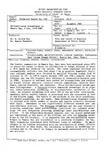
The mean annual blue (irrigation) water requirement computed by the GCWM was 1181 km3 for the period 1998 – 2002. The related green (precipitation) water use of crops on irrigated land was 919 km3 yr-1. Thus the computed blue water requirement accounts for 56.2 % of the global crop water use on irrigated land. Since the total harvested area of irrigated crops was about 312 Mha (Portmann et al., 2008), the blue water requirement was 378 mm yr-1 on average related to the harvested crop area. Irrigation water requirements per 30 arc minute cell are shown in Figure 4a. Near the equator one 30 arc minute by 30 arc minute cell covers an area of about 2400 km2. In Figure 4a high irrigation requirements appear for areas with a high density of irrigated areas, a high cropping intensity on irrigated land and additionally a large climatic water deficit during the growing season. Those areas were for example located in the Punjab region in Pakistan and India, the Nile delta in Egypt and in parts of California. Irrigation water requirements were more than 1000 mm yr-1 in grid cells belonging to these regions. Irrigation water requirements related to the actually used irrigated area of the 30 arc minute grid cells are shown in Figure 4b. In this representation, the absolute values of water use are independent of the density of irrigated areas in the grid cell. High values of more than 1000 mm yr-1 were found for all arid regions on the globe, e.g. the Western United States, North-East Brazil, along the west coast of South America, in the Near East region, South Asia, Australia and the non-tropical regions of Africa. The percentage of crop evapotranspiration on irrigated land met by blue water (Figure 4c) shows a typical gradient from less than 10 % in temperate, humid regions (e.g. Scandinavia, Alaska) to 10 – 30 % in Central Europe, the Eastern United States and Southern China, 30 – 60 % in regions like Northern Spain, Northern Italy or along the East coast of Australia and more than 60 % in semi-arid and arid regions. The largest crop-specific irrigation water requirements were simulated for rice (308 3 -1 km yr ), wheat (208 km3 yr-1), managed grassland (90 km3 yr-1), maize (84 km3 yr-1), other perennial crops (84 km3 yr-1) and cotton (83 km3 yr-1). These are also the crops that have the largest harvested areas on irrigated land (Table 3). For rice, irrigation water requirements (related to the total 30 arc minute grid cell area) of more than 100 mm yr-1 were computed for the Ganges, Brahmaputra and Indus basins in India, Bangladesh and Pakistan, the Eastern part of China, the island of Java (Indonesia), the Nile delta in Egypt and the lower Mississippi in the United States (Figure 5a). For wheat, the largest irrigation water requirements on that scale were computed for the Indus basin, the whole North-Western part of India and along the Nile river in Egypt (Figure 5b). The irrigation water requirements for maize were largest for the Great Plains in the United States, along the Nile river in Egypt and for the coastal plain southeast of Peking in China (Figure 5c). The global average of the irrigation water requirement related to the harvested area of the crop was largest for date palms (1428 mm yr1 ), managed grassland (771 mm yr-1) and sugar cane (673 mm yr-1). The percentage of crop water use provided as irrigation water was largest for date palms (89 %) and sugar beets (75 %). Low percentages of crop water use provided as irrigation water were computed for cocoa and oil palms (Table 3) which indicates that these crops are growing in more humid

The Global Crop Water Model (GCWM) – Results

20

(a)

(b)

(c)

FIGURE 4 Mean blue water requirement during period 1998 – 2002 related to total cell area of 30 arc minute cells in mm yr-1 (a), mean blue water requirement during period 1998 – 2002 related to the used irrigated area of 30 arc minute cells in mm yr-1 (b) and percentage of total crop evapotranspiration on irrigated cropland from blue (irrigation) water (c).


21

(a)

(b)

(c)

FIGURE 5 Mean blue water requirement during period 1998 – 2002 related to total cell area of 30 arc minute cells in mm yr-1 for rice (a), wheat (b) and maize(c).


22

regions or that irrigation water is only required to balance out water deficits in a relatively short part of the growing season. At the global scale, the largest blue water requirements of crops were computed for the months July and August. The two months accounted for about 25 % of the total irrigation water requirements (Figure 6). However, the seasonality of irrigation water requirements depends on the specific crop and the location of the growing area of the crop, mainly its TABLE 3 Irrigated area harvested (IAH) in ha yr-1, total irrigation water requirement (IWRtot) in km3 yr-1, crop water use from green water (CWUgreen) in km3 yr-1, irrigation water requirement related to IAH (IWRIAH) in mm yr-1 and percentage of crop evapotranspiration from irrigation water (IWRfrac) computed for irrigated land by using the Global Crop Water Model (GCWM) in the period 1998 – 2002. IAH*

Crop

-1

IWRtot 3

-1

CWUgreen 3

-1

IWRIAH -1

IWRfrac

(ha yr )

(km yr )

(km yr )

(mm yr )

(%)

Wheat

66,632,207

207.9

115.4

312

64

Maize

29,900,725

84.2

98.1

282

46

Rice

103,119,735

307.8

337.1

298

48

Barley

4,645,845

10.9

8.5

234

56

Rye

442,272

1.0

1.2

232

45

Millet

1,743,732

4.0

4.3

227

48

Sorghum

3,436,564

10.8

10.0

313

52

Soybeans

6,032,662

17.3

25.0

287

41

Sunflower

1,268,735

4.1

3.5

322

54

Potatoes

3,745,495

13.3

8.5

356

61

Cassava

11,194

0.0

0.0

273

48

Sugar cane

10,189,040

68.6

70.9

673

49

Sugar beets

1,574,017

9.1

3.0

575

75

Oil palm

11,000

0.0

0.1

435

32

Rapeseed / canola

3,403,812

7.9

3.0

231

73

Groundnuts / peanuts

3,675,801

7.5

13.1

204

36

Pulses

5,455,809

22.4

7.7

411

75

Citrus

3,562,670

22.6

17.8

634

56

Date palm

723,436

10.3

1.3

1428

89

Grapes / vine

1,726,682

7.0

5.0

407

58

Cotton

16,252,239

82.9

46.8

510

64

Cocoa

12,544

0.0

0.1

258

20

Coffee

173,916

1.1

1.4

643

44

Others (perennial)

12,852,976

84.2

55.9

655

60

Managed grassland / pasture

11,684,004

90.1

47.0

771

66

Fallow**

20,138,732 n.a.

62.2 43.2

34.2 0.0

309 n.a.

65 n.a.

Total

312,431,073

1181.525

915.737

378

56

Others (annual)

*: **:

It was assumed that perennial crops, sugar cane and grassland / pasture are harvested once in a year. In the fallow or rainfed period after the harvesting irrigated crops there is still blue water stored in the soil which can go into evapotranspiration. Since the specific crop rotation within the grid cells is unknown, evapotranspiration of blue water in the rainfed period cannot be attributed to a specific crop and appears therefore summarized in the fallow category.


23

latitude (Figures B3 – B5 in the appendix). The largest irrigation water requirements for wheat were computed for the months March and April, while for rice the largest irrigation water requirement were simulated for the period June – September. Compared to wheat, the irrigation water use for rice was found to be much more balanced between the different months (Figure 6). The largest irrigation water requirements at the country scale were computed for India (287 km3 yr-1), China (147 km3 yr-1), the United States (139 km3 yr-1) and Pakistan (117 km3 yr-1). These countries account for 58 % of the global irrigation water requirements (Table A1 in the appendix). Irrigation water requirements of more than 1 km3 yr-1 were simulated for 59 countries. The largest irrigation requirements related to the irrigated area harvested were calculated for the Arabian countries United Arab Emirates (1616 mm yr-1), Oman (1461 mm yr-1), Bahrain (1272 mm yr-1), Saudi Arabia (967 mm yr-1), Qatar (879 mm yr-1) and Kuwait (858 mm yr-1), for the North-African countries Mauritania (864 mm yr-1), Libya (847 mm yr1 ), Sudan (836 mm yr-1) and Egypt (779 mm yr-1) and for the Near East countries Iraq (855 mm yr-1), Israel (835 mm yr-1) and Jordan (775 mm yr-1). The lowest irrigation water requirements related to irrigated area harvested were computed for small islands like Northern Marianna Islands and Guam (0 mm yr-1), but also for some European countries like Switzerland (6 mm yr-1), Denmark (23 mm yr-1) and Ireland (41 mm yr-1). The fraction of total crop water use required as blue water was largest for Egypt and the Arabian countries Bahrain, United Arab Emirates, Qatar, Oman, Saudi Arabia and Kuwait (for all larger than 93 %). For 39 countries the blue water requirement was larger than 70 % of the total crop water use on irrigated land. On the other hand the percentage of green water use was larger than 70 % for 58 countries indicating the importance of stored precipitation water even on irrigated land. 160 140

Wheat Rice

120

3

-1

Irrigation water requirement (km month )

Others

100 80 60 40 20 0 JAN

FEB

MAR

APR

MAY

JUN

JUL

AUG

SEP

OCT

NOV

DEC

Month

FIGURE 6 Mean monthly blue water requirements during period 1998 – 2002 for rice, wheat and the other crops in km3 month-1.

The Global Crop Water Model (GCWM) – Discussion

4

24

DISCUSSION

The model presented here should be considered as a first attempt to simulate green and blue water use on cropland. It is necessary to analyze the uncertainty of the model and to check the sensitivity to changes of the most important parameters in a systematic way. Several sources of uncertainty were already identified. These are: the data set on monthly crop growing areas and the related cropping calendars the parameters used to compute daily crop coefficients (kc) the methodology to compute reference evapotranspiration and the spatial and temporal resolution of the used climate input data. A systematic uncertainty analysis of the model will be the objective of further research. Here we present first results of a comparison of model results to statistical information and to results of other models. 4.1

Comparison of the simulated irrigation water requirements to census-based statistical information The interpretation of a comparison of simulated results for irrigation water requirement to census-based statistical information is difficult because published statistics usually refer to irrigation water withdrawals. These withdrawals are larger than the crop water requirements because a significant part of the water withdrawn from its source goes into unproductive losses (e.g. evaporation and leakage in canals on the way to the field, percolation losses in the field). On the other hand the irrigation water requirements computed by the model refer to the amount of water that would potentially be needed to ensure optimal plant growing. In many cases farmers decide because of several reasons (e.g. water shortages, high costs for water, electricity and labour, damaged infrastructure, labour peaks) to provide a lower amount of water to the plants and to practice so called deficit irrigation. These limitations have to be taken into account when interpreting the comparisons in the following two sections to data on irrigation water withdrawals for European countries and to consumptive water uses in the federal states of the United States of America. Because of the well established quality standards in the statistical reporting system in the European Union and the United States these two sources of information are assumed to be relatively reliable compared to statistics in other countries. Comparison of model results to statistics on irrigation withdrawal water use in European countries The statistics used here were collected by EUROSTAT from national sources and refer to total annual surface and groundwater abstraction of agriculture for irrigation purposes (EUROSTAT, 2007). We computed averages for the years 1998 – 2002 if data were available for these years (Table 4). In some cases however, we had to consider older statistics because of missing data. Therefore the reference years for the statistics are also listed. The comparison shows that the computed irrigation water requirements are lower than the reported withdrawals and reasonable for most of the countries that reported large irrigation water uses,


25

e.g. Turkey, Spain, Greece, Portugal, Bulgaria, Germany, Netherlands and Denmark. But also for some countries, which reported low irrigation water withdrawals, the computed results were in the expected range, e.g. for Sweden, Austria, Finland and Lithuania. GCWM simulated too high irrigation water requirements for Romania, Hungary, England and Wales, Poland, Slovakia, the Czech Republic and Slovenia while it simulated to less irrigation water requirements for Norway. The differences for the Eastern European countries maybe explained by incorrect model inputs related to irrigated areas and irrigated crops. It was already mentioned elsewhere (Siebert et al., 2006) that the data on irrigated area for these countries are uncertain because of the ongoing restructuring of the irrigation sector. Additionally, it was also reported, that actual water withdrawals for irrigation are much lower than the requirements (e.g. for Romania in Nicolaescu et al., 2005). The differences for Norway were surprising because the results for the other Scandinavian countries fitted well to the expected irrigation water requirements based on the statistics. Thus there is a need for further investigations to find the reasons for it. TABLE 4 Reference years of the statistics and of the model output, irrigation withdrawal use (IWU) reported by the EUROSTAT statistics in Mm3 yr-1 and irrigation water requirement (IWR) as simulated by the Global Crop Water Model (GCWM) in Mm3 yr-1 and the ratio between the simulated IWR and IWU.

Reference year(s) EUROSTAT

Reference year(s) GCWM

Turkey

1997 - 2001

Spain Greece

Country

IWU EUROSTAT (Mm3 yr-1)

IWR GCWM (Mm3 yr-1)

IWR / IWU (-)

1998 - 2002

28,480.8

14,628.7

0.51

1998 - 2002

1998 - 2002

22,530.6

18,631.1

0.83

1997

1998 - 2002

7,600.0

6,930.4

0.91

Portugal

1998

1998

6,550.9

3,269.6

0.50

Romania

1998 - 2002

1998 - 2002

574.8

900.3

1.57

Bulgaria

1998 - 2002

1998 - 2002

486.6

120.8

0.25

Germany

1998, 2002

1998, 2002

152.7

146.3

0.96

Netherlands

1995 - 1999

1998 - 2002

141.8

123.4

0.87

Denmark

1995

1998 - 2002

140.0

47.3

0.34

Norway

1998 - 2002

1998 - 2002

129.3

15.1

0.12

Hungary

1998 - 2002

1998 - 2002

121.6

206.1

1.69

England and Wales

1997 - 2001

1998 - 2002

119.7

214.1

1.79

Sweden

1998 - 2002

1998 - 2002

101.8

47.9

0.47

Poland

1998 - 2002

1998 - 2002

97.2

103.8

1.07

Austria

1995 - 1999

1998 - 2002

66.4

34.6

0.52

Slovakia

1998 - 2002

1998 - 2002

47.9

191.2

3.99

Finland

1999

1999

40.0

19.4

0.49

Czech Republic

1998 - 2002

1998 - 2002

8.1

20.6

2.55

Lithuania

2003

1998 - 2002

6.6

3.1

0.48

5.6 < 0.1

0.99 0.09

Slovenia

1995, 2002

1998 - 2002

5.7

Luxembourg

1995

1998 - 2002

0.2


26

Comparison of model results to statistics on irrigation consumptive water use in the United States of America The computed irrigation water requirements were compared to published information on irrigation consumptive use (Hutson et al., 2004; Solley et al., 1998) on the level of the federal states. Because the water census undertaken in year 2000 (Hutson et al., 2004) only collected data on irrigation withdrawal uses, irrigation consumptive use was computed for each federal state by applying the ratio between irrigation consumptive use and irrigation withdrawal use published for the water census 1995 (Solley et al., 1998). It was found, that there is in general a reasonable agreement between the values computed by the GCWM and the published census data (Figure 7). On the level of federal states the two data sets were correlated with a r2 of 0.85, the modeling efficiency according to Nash and Sutcliffe (1970) was 0.82. In general, computed irrigation water requirements were larger than reported water consumption for all the states in the centre of the country (Texas, Louisiana, New Mexico, Oklahoma, Arkansas, Kansas, Nebraska, Colorado). A first analysis indicated that the large wind speeds reported for this area caused a relatively high reference evapotranspiration computed using the Penman-Monteith approach while the differences became much lower when using the Priestley-Taylor equation to compute ET0 (r2 of 0.94, Nash-Sutcliffe coefficient 0.93). The irrigation water requirement computed by the GCWM for the total United States and year 2000 (147.8 km3 yr-1) was also larger than the reported consumptive water use of 117.3 km3 yr-1. Further research is therefore needed to identify the specific reasons for the differences. 100,000

10,000

1,000

100

10

1 0

0 0.1

1

10

100

1,000

10,000

100,000

0.10

0 ICU USGS (Mm3 yr-1)

FIGURE 7 Irrigation consumptive water use according to the USGS statistics (ICU USGS) and irrigation water requirements computed by the Global Crop Water Model (GCWM) for the reference year 2000 in federal states of the United States in Mm3 yr-1.


27

4.2

Comparison of the simulated irrigation water requirements to agricultural water use and irrigation water requirement reported by FAO for 90 developing countries In the following section we compare the irrigation water requirements modeled using the GCWM to those modeled by the Food and Agriculture Organization of the United Nations (FAO) and to total agricultural water withdrawals reported in the FAO AQUASTAT database. The FAO used a crop water model that is also based on a soil water balance and the mean climate 1961-90 (New et al., 1999) as climate input (FAO, 2005). The land use was based on a previous version of the Digital Global Irrigation Map (Siebert et al., 2001) and cropping calendars from an earlier version of the FAO AQUASTAT database. The total irrigation water requirement of the 90 developing countries computed by FAO was 824 km3 yr-1, while the corresponding irrigation water requirement of GCWM was 902 km3 yr-1. It was found that the irrigation water requirements simulated by GCWM were larger for many arid countries (Table 5). For countries, in which rice is the dominating irrigated crop, FAO computed larger values (e.g. for Indonesia, Vietnam, Myanmar, Philippines). The reason maybe that FAO assumed for rice cultivation an additional irrigation water requirement of 250 mm at the beginning of the growing season to flood the paddy fields (FAO, 2005). TABLE 5 Agricultural water withdrawal use (AWWU) in km3 yr-1, irrigation water requirement as computed by FAO (IWRFAO) and by the Global Crop Water Model (IWRGCWM) in km3 yr-1, ratio between IWRGCWM and AWWU (only developing countries with an AWWU of more than 4 km3 yr-1 are shown in the table).

Country

AWWU 3

-1

IWRFAO 3

-1

IWRGCWM 3

-1

IWRGCWM / AWWU

(km yr )

(km yr )

(km yr )

(-)

India

558.00

303.24

286.97

0.51

China

427.00

153.90

147.22

0.34

Pakistan

163.00

72.14

117.04

0.72

Thailand

82.80

24.83

19.09

0.23

Bangladesh

76.40

19.09

18.67

0.24

Indonesia

75.60

21.49

13.58

0.18

Iran, Islamic Rep of

66.20

21.06

40.78

0.62

Mexico

60.30

18.53

26.80

0.44

Egypt

59.00

28.43

46.92

0.80

Viet Nam

48.60

15.18

7.41

0.15

Iraq

39.40

11.20

20.86

0.53

Brazil

36.60

6.21

8.34

0.23

Sudan

36.10

14.43

10.09

0.28

Myanmar

32.60

9.79

5.92

0.18

Turkey

27.90

11.27

14.63

0.52

Afghanistan

22.80

8.78

9.44

0.41

Argentina

21.50

3.43

5.75

0.27

Philippines

21.10

6.33

3.80

0.18

Syrian Arab Republic

18.90

8.52

9.46

0.50


Country

AWWU 3

-1

28

IWRFAO 3

-1

IWRGCWM 3

-1

IWRGCWM / AWWU

(km yr )

(km yr )

(km yr )

(-)

Peru

16.40

5.07

5.07

0.31

Saudi Arabia

15.40

6.68

12.38

0.80

Madagascar

14.30

3.58

2.81

0.20

Ecuador

14.00

2.67

2.72

0.19

Sri Lanka

12.00

2.92

2.22

0.19

Morocco

11.00

4.28

8.97

0.82

Nepal

9.82

2.45

4.20

0.43

Korea, Republic of

8.92

2.67

0.84

0.09

Chile

7.97

1.59

3.00

0.38

South Africa

7.84

2.34

8.81

1.12

Yemen

6.32

2.53

2.93

0.46

Mali

5.90

2.06

1.27

0.21

Cuba

5.64

1.41

1.62

0.29

Malaysia

5.60

1.68

0.62

0.11

Nigeria

5.51

1.65

0.89

0.16

Ethiopia

5.20

0.56

1.19

0.23

Korea, Dem. Rep.

4.96

1.49

1.10

0.22

Colombia

4.92

1.23

0.96

0.20

Tanzania

4.63

0.56

0.98

0.21

4.00 2101.12

1.20 824.21

1.04 902.02

0.26 0.43

Cambodia All 90 countries

5

SUMMARY AND CONCLUSIONS

The presented global crop water model was developed to compute blue (irrigation) water requirements and crop evapotranspiration from green (precipitation) water at a spatial resolution of 5 arc minutes by 5 arc minutes for 26 different crops. The model is based on soil water balances performed for each crop and each grid cell. For the first time a new global data set was applied consisting of monthly growing areas for these 26 crops and related cropping calendars. Crop water use was computed for the period 1998 – 2002. First results for irrigated cropland are presented in this report. The global irrigation water requirement in the reference period was 1181 km3 yr-1 while the green water use of irrigated crops was 919 km3 yr-1. At the global scale the largest irrigation water requirement was computed for rice, wheat, managed grassland, maize and sugar cane. The percentage of crop water use provided as irrigation water was largest for date palms and sugar beets while for cocoa and oil palms green water use was dominant. The countries with the largest irrigation water requirements were India, China, the United States and Pakistan. A strong seasonal variation of irrigation water requirements was observed with maximum monthly values for July and August. A comparison of the model results for irrigated crops to external statistical information and to results of other models showed a reasonable agreement for most countries in Europe, many of the federal states in the US and the most developing countries. These first

The Global Crop Water Model (GCWM) – Summary and conclusions

29

comparisons clearly indicated the need for a systematic validation of the model including an uncertainty and sensitivity analysis. As soon as the data set of monthly crop growing areas also includes rainfed crops, the model will be applied to compute the green water use of rainfed crops to provide consistent figures for the whole crop water use. The modeling results will be made available to the public via the web site of the "virtual water project" at http://www.geo.unifrankfurt.de/ipg/ag/dl/forschung/Virtual_water/index.html.

The Global Crop Water Model (GCWM) – References

30

REFERENCES Alcamo, J., Döll, P., Henrichs, T., Kaspar, F., Lehner, B., Rösch, T. & Siebert, S. (2003a): Global estimates of water withdrawals and availability under current and future "business-as-usual" conditions. Hydrological Sciences Journal, 48(3), 339-348. Alcamo, J., Döll, P., Henrichs, T., Kaspar, F., Lehner, B., Rösch, T. & Siebert, S. (2003b): Development and testing of the WaterGAP 2 global model of water use and availability. Hydrological Sciences Journal, 48(3), 317-338. Alcamo, J., Döll, P., Kaspar, F. & Siebert, S. (1997): Global change and global scenarios of water use and availability: An application of WaterGAP 1.0, Report A9701, Center for Environmental Systems Research, University of Kassel, Germany, 47 pp + Appendix. Allan, J.A. (1993) ‘Fortunately there are substitutes for water otherwise our hydro-political futures would be impossible’ In: Priorities for water resources allocation and management, ODA, London, pp. 13-26. Allen, R. G., Pereira, L. S., Raes, D. & Smith, M. (1998): Crop evapotranspiration - Guidelines for computing crop water requirements. FAO Irrigation and Drainage Paper 56, Rome, Italy. Batjes, N. H. (2006): ISRIC-WISE derived soil properties on a 5 by 5 arc-minutes global grid. Report 2006/02 (available through http://www.isric.org), ISRIC – World Soil Information, Wageningen, The Netherlands, (with data set). Chapagain, A. K. & Hoekstra, A. Y. (2004): Water footprints of nations. Value of Water Research Report Series No. 16, UNESCO-IHE, Delft, The Netherlands. Chapagain, A.K., Hoekstra, A.Y., & Savenije, H.H.G. (2006): Water saving through international trade of agricultural products. Hydrology and Earth System Sciences 10 (3), 455-468. Döll, P., Kaspar, F. & Lehner, B. (2003): A global hydrological model for deriving water availability indicators: model tuning and validation. Journal of Hydrology, 270 (1-2), 105-134. Döll, P. & Siebert, S. (2002): Global modeling of irrigation water requirements. Water Resources Research, 38(4), 8.1-8.10, DOI 10.1029/2001WR000355. EUROSTAT (2007): Annual water abstraction by source and by sector. Online database, available at: http://epp.eurostat.ec.europa.eu/portal/page?_pageid=1073,46870091&_dad=portal&_schema=PORTA L&p_product_code=ENV_WATQ2_1. FAO (2007): AQUASTAT data base. FAO, Rome, Italy, available at: http://www.fao.org/ag/agl/aglw/ aquastat/main/index.stm. FAO (2005): Review of agricultural water use per country. Online publication, FAO, Rome, Italy, available at: http://www.fao.org/ag/agl/aglw/aquastat/water_use/index.stm. Forsythe, W.C., Rykiel, E.J., Stahl, R.S., Wu, H. & Schoolfield, R.M. (1995): A model comparison for daylength as a function of latitude and day of year. Ecol. Model. 80, 87–95. Geng, S., Penning, F. W. T. & Supit, I. (1986): A simple method for generating daily rainfall data, Agric. For. Meteorol., 36, 363–376. Hutson, S. S., Barber, N. L., Kenny, J. F., Linsey, K. S., Lumia, D. S. & Maupin, M. A. (2004): Estimated use of water in the United States in 2000. U.S. Geological Survey circular 1268, Reston, United States, available at: http://water.usgs.gov/watuse/. Lehner, B., Döll, P., Alcamo, J., Henrichs, H. & Kaspar, F. (2006): Estimating the impact of global change on flood and drought risks in Europe: a continental, integrated analysis. Climatic Change, 75, 273–299. DOI: 10.1007/s10584-006-6338-4.

The Global Crop Water Model (GCWM) – References

31

Mitchell, T. D. & Jones, P. D. (2005): An improved method of constructing a database of monthly climate observations and associated high-resolution grids. International Journal of Climatology, 25, 693-712. Nash, J. E. & Sutcliffe, J. V. (1970): River flow forecasting through conceptual models, Part I – A discussion of principles. Journal of Hydrology 10, 282-290. New, M., Hulme, M. & Jones, P. (1999): Representing Twentieth-Century Space-Time Cimate Variability. Part I: Development of a 1961-90 Mean Monthly Terrestrial Climatology in "Journal of Climate" Volume 12, March 1999. New, M., Lister, D., Hulme, M. & Makin, I. (2002): A high-resolution data set of surface climate over global land areas. Climate Research, 21(1), 1-25. Nicolaescu, I., Buhociu, L., Condruz, R., Suciu, G.-I., Paraschiv, D. & Boeru, M. (2006): Country report from Romania. In: Dirksen, W. and Huppert, W. (ed.). Irrigation sector reform in Central and Eastern European countries. Deutsche Gesellschaft für Technische Zusammenarbeit (GTZ), Eschborn, Germany, 385-462. NOAA (1988): Data Announcement 88-MGG-02, Digital relief of the Surface of the Earth. NOAA, National Geophysical Data Center, Boulder, Colorado. Oki, T. & Kanae, S. (2004), Virtual water trade and world water resources, Water Science & Technology, 49 (7), 203-209. Portmann, F., Siebert, S., Bauer, C. & Döll, P. (2008): Global data set of monthly growing areas of 26 irrigated crops. Frankfurt Hydrology Paper 06, Institute of Physical Geography, University of Frankfurt, http://www.geo.uniFrankfurt am Main, Germany, available at: frankfurt.de/fb/fb11/ipg/ag/dl/f_publikationen/2007/FHP_06_Portmann_et_al_2008.pdf Press, W. H., Flannery, B. P., Teukolsky, S. A. & Vetterling, W. T. (1992): Numerical recipes in C: the art of scientific computing. Cambridge University Press, 994 pp. Priestley, C., & Taylor, R. (1972): On the assessment of surface heat flux and evaporation using large scale parameters, Mon. Weather Rev., 100, 81– 92. Seckler, D., Amarasinghe, U., Molden, D., De Silva, R. & Barker, R. (2000): World water demand and supply 1990 to 2025: scenarios and issues. IWMI Research Report 19, IWMI, Colombo, Sri Lanka, 40 pp. Shiklomanov, I. A. (2000): Appraisal and assessment of world water resources. Water International, 25(1), 1132. Shuttleworth, W. J. (1993): Evaporation, in Handbook of Hydrology, edited by D. R. Maidment, pp. 4.1–4.53, McGraw-Hill, New York. Siebert, S., Hoogeveen, J. & Frenken, K. (2006): Irrigation in Africa, Europe and Latin America. Update of the Digital Global Map of Irrigation Areas to Version 4. Frankfurt Hydrology Paper 05, Institute of Physical Geography, Frankfurt University, Frankfurt am Main, Germany, 134 pp. Siebert, S., Döll, P. & Hoogeveen, J. (2002): Global map of irrigated areas version 2.1. Center for Environmental Systems Research, University of Kassel, Germany, and FAO, Rome, Italy. Solley, W. B., Pierce, R. R. & Perlman, H. A. (1998): Estimated use of water in the United States in 1995. U.S. Geological Survey circular 1200, Denver, United States, available at: http://water.usgs.gov/watuse/. Vörösmarty, C. J., Green, P., Salisbury, J. & Lammers, R. B. (2000): Global water resources: vulnerability from climate change and population growth. Science, 289, 284–288. Yang, H., Wang, L., Abbaspour, K.C. & Zehnder, A.J.B. (2006): Virtual water highway: water use efficiency in global food trade. Hydrology & Earth System Sciences 3, 1–26.

The Global Crop Water Model (GCWM) – Annex A - Tables

Annex A - Tables

32


33

TABLE A1 Irrigated area harvested (IAH) in ha yr-1, total irrigation water requirement (IWRtot) in km3 yr-1, crop water use from green water (CWUgreen) in km3 yr-1, irrigation water requirement related to IAH (IWRIAH) in mm yr-1 and percentage of crop evapotranspiration from irrigation water (IWRfrac) computed for irrigated land by using the Global Crop Water Model (GCWM) in the period 1998 – 2002 (only countries with irrigated area are listed).

Country

IAH* -1

Afghanistan Albania Algeria Andorra Angola Antigua and Barbuda Argentina Armenia Australia Austria Azerbaijan Bahrain Bangladesh Barbados Belarus Belgium Belize Benin Bhutan Bolivia Bosnia and Herzegovina Botswana Brazil Brunei Bulgaria Burkina Faso Burundi Cambodia Cameroon Canada Cape Verde Central African Republic Chad Chile China Colombia Comoros Congo, Dem. Rep. Congo, Rep Costa Rica Cote D'Ivoire Croatia Cuba Cyprus Czech Republic Denmark Djibouti Dominican Republic Ecuador Egypt

(ha yr ) 1,912,917 180,000 570,447 150 42,000 130 1,352,379 172,806 2,384,292 41,076 730,129 3,113 6,431,077 1,000 115,000 10,378 3,000 2,823 43,507 127,001 3,000 620 2,820,954 1,000 50,898 20,233 20,130 336,992 45,079 707,053 2,578 69 26,804 897,274 85,655,033 645,000 85 7,771 2,000 123,030 41,618 5,000 822,225 36,210 16,554 204,071 388 220,000 686,000 6,027,115

IWRtot 3

-1

(km yr ) 9.4401 0.7415 4.2781 0.0003 0.2059 0.0001 5.7517 0.5967 13.6380 0.0346 3.8453 0.0396 18.6735 0.0017 0.1522 0.0050 0.0044 0.0132 0.0573 0.4168 0.0110 0.0037 8.3360 0.0006 0.1208 0.1268 0.0690 1.0450 0.2055 2.7152 0.0104 0.0001 0.1404 2.9951 147.2152 0.9615 0.0003 0.0234 0.0045 0.4344 0.1405 0.0097 1.6176 0.2753 0.0206 0.0473 0.0025 0.9041 2.7200 46.9247

CWUgreen 3

-1

(km yr ) 2.5582 0.6305 0.9566 0.0004 0.1068 0.0007 5.7290 0.3068 10.8816 0.1502 1.1763 0.0007 24.3373 0.0050 0.4952 0.0289 0.0201 0.0134 0.2269 0.3346 0.0106 0.0016 18.0386 0.0067 0.1265 0.0730 0.0771 1.7786 0.1567 2.3464 0.0113 0.0003 0.1008 2.0670 256.7833 3.6763 0.0008 0.0522 0.0148 0.8682 0.3253 0.0210 6.2182 0.0765 0.0727 0.5123 0.0005 1.5057 2.1122 0.7647

IWRIAH -1

(mm yr ) 493 412 750 182 490 67 425 345 572 84 527 1272 290 169 132 48 145 468 132 328 368 595 296 56 237 627 343 310 456 384 405 170 524 334 172 149 295 301 223 353 338 195 197 760 125 23 641 411 397 779

IWRfrac

(%) 79 54 82 39 66 12 50 66 56 19 77 98 43 25 24 15 18 50 20 55 51 70 32 8 49 63 47 37 57 54 48 32 58 59 36 21 23 31 23 33 30 32 21 78 22 8 84 38 56 98


Country

IAH* -1

El Salvador Eritrea Estonia Ethiopia Fiji Finland France French Guyana Gabon Gambia Georgia Germany Ghana Greece Grenada Guadeloupe Guam Guatemala Guinea Guinea Bissau Guyana Haiti Honduras Hungary India Indonesia Iran Iraq Ireland Israel Italy Jamaica Japan Jordan Kazakhstan Kenya Korea, Democratic People's Republic of Korea, Republic of Kuwait Kyrgyzstan Laos Latvia Lebanon Lesotho Liberia Libya Lithuania Luxembourg Macedonia Madagascar Malawi Malaysia Mali Malta Martinique Mauritania Mauritius Mexico

IWRtot 3

-1

34

CWUgreen 3

-1

IWRIAH -1

IWRfrac

(ha yr ) 50,710 5,969 600 410,557 3,000 20,000 1,708,020 6,007 8,450 2,149 196,702 266,827 17,138 1,237,967 218 5,697 312 139,788 20,386 8,562 178,029 89,000 100,000 103,764 68,724,872 7,108,333 7,296,524 2,439,000 1,100 184,072 2,670,358 24,666 2,167,228 100,105 1,804,753 76,813

(km yr ) 0.2107 0.0390 0.0004 1.1919 0.0003 0.0095 3.2194 0.0081 0.0124 0.0104 0.4917 0.2113 0.0518 6.9304 0.0004 0.0043 0.0000 0.6541 0.0698 0.0538 0.3284 0.2322 0.3605 0.2061 286.9738 13.5840 40.7829 20.8607 0.0005 1.5371 6.4612 0.0546 1.6519 0.7760 8.8560 0.4549

(km yr ) 0.2543 0.0131 0.0023 1.4011 0.0145 0.0594 6.0108 0.0325 0.0260 0.0065 0.6376 0.9083 0.0513 2.4991 0.0008 0.0651 0.0017 1.2307 0.0917 0.0485 1.2397 0.5105 0.5626 0.3819 174.9560 43.2047 10.6871 2.1195 0.0039 0.1554 8.7693 0.2684 9.0626 0.0754 3.1984 0.3322

(mm yr ) 415 653 71 290 8 48 188 135 147 482 250 79 302 560 181 76 0 468 342 628 184 261 360 199 418 191 559 855 41 835 242 221 76 775 491 592

(%) 45 75 16 46 2 14 35 20 32 61 44 19 50 73 32 6 0 35 43 53 21 31 39 35 62 24 79 91 10 91 42 17 15 91 73 58

1,278,000 875,415 8,509 1,140,614 354,642 833 139,292 203 2,100 316,000 4,416 24 42,500 1,105,685 56,515 501,606 180,317 3,540 6,730 23,084 20,919 5,958,094

1.1048 0.8358 0.0730 3.1238 1.2797 0.0007 0.9677 0.0004 0.0029 2.6761 0.0031 0.0000 0.1915 2.8126 0.3440 0.6150 1.2675 0.0144 0.0128 0.1996 0.0789 26.8002

5.5678 4.0216 0.0039 2.5500 1.4057 0.0026 0.2213 0.0003 0.0075 0.2874 0.0149 0.0000 0.1254 4.3617 0.3542 2.8419 0.3980 0.0043 0.0776 0.0437 0.2031 24.2360

86 95 858 274 361 81 695 200 140 847 71 72 451 254 609 123 703 407 190 864 377 450

17 17 95 55 48 20 81 62 28 90 17 26 60 39 49 18 76 77 14 82 28 53


Country

IAH* -1

Moldova Republic of Mongolia Montenegro Morocco Mozambique Myanmar Namibia Nepal Netherlands New Zealand Nicaragua Niger Nigeria Northern Mariana Islands Norway Oman Pakistan Palestine (Gaza Strip and West Bank) Panama Paraguay Peru Philippines Poland Portugal Puerto Rico Qatar Reunion Romania Russian Federation Rwanda Saint Kitts and Nevis Saint Lucia Sao Tome and Principe Saudi Arabia Senegal Serbia (including Kosovo) Seychelles Sierra Leone Slovakia Slovenia Somalia South Africa Spain Sri Lanka Sudan Suriname Swaziland Sweden Switzerland Syria Taiwan, Province of China Tajikistan Tanzania Thailand Timor Leste (East Timor) Togo Trinidad and Tobago Tunisia

IWRtot 3

-1

35

CWUgreen 3

-1

IWRIAH -1

IWRfrac

(ha yr ) 256,377 57,300 2,109 1,468,600 40,063 2,263,062 8,806 1,257,984 153,650 383,236 75,222 96,125 164,000 60 36,200 72,461 19,344,802

(km yr ) 0.7089 0.2965 0.0048 8.9690 0.1681 5.9249 0.0672 4.2003 0.1234 0.6842 0.3338 0.6165 0.8873 0.0000 0.0151 1.0588 117.0439

(km yr ) 0.6355 0.0866 0.0084 2.2344 0.2393 6.5030 0.0187 3.9909 0.7749 2.1011 0.4115 0.2079 0.6452 0.0004 0.1416 0.0639 19.2518

(mm yr ) 277 518 229 611 419 262 764 334 80 179 444 641 541 0 42 1461 605

(%) 53 77 36 80 41 48 78 51 14 25 45 75 58 0 10 94 86

29,197 30,811 54,000 1,108,999 2,067,000 83,292 638,947 17,465 9,544 7,584 422,724 3,772,922 5,500 18 297 9,700 1,280,725 83,904 60,071 224 30,000 104,560 10,324 206,000 1,664,300 3,423,510 731,700 1,208,110 51,180 45,482 53,440 14,500 1,507,867 588,798 637,213 227,000 6,187,300 7,000 2,557 3,600 367,000

0.2018 0.0598 0.0894 5.0700 3.7971 0.1038 3.2463 0.0432 0.0839 0.0077 0.9003 11.6267 0.0118 0.0000 0.0005 0.0186 12.3795 0.6041 0.1580 0.0005 0.1167 0.1912 0.0056 0.9809 8.8129 18.6311 2.2227 10.0950 0.0941 0.2656 0.0479 0.0009 9.4585 0.6837 3.2782 0.9838 19.0901 0.0123 0.0120 0.0090 2.5949

0.0171 0.2911 0.4984 1.4412 10.3969 0.3219 1.8630 0.1926 0.0023 0.0599 1.2530 13.3821 0.0167 0.0001 0.0030 0.1048 0.7229 0.2002 0.2441 0.0008 0.1091 0.3658 0.0476 0.6510 6.4502 9.1600 2.9985 2.8930 0.3144 0.3088 0.2028 0.0414 2.1962 2.6261 1.0146 0.8119 30.8103 0.0443 0.0146 0.0363 0.7089

691 194 166 457 184 125 508 248 879 101 213 308 214 59 179 191 967 720 263 217 389 183 55 476 530 544 304 836 184 584 90 6 627 116 514 433 309 176 469 250 707

92 17 15 78 27 24 64 18 97 11 42 46 41 14 15 15 94 75 39 39 52 34 11 60 58 67 43 78 23 46 19 2 81 21 76 55 38 22 45 20 79


Country

IAH* -1

Turkey Turkmenistan Uganda Ukraine United Arab Emirates United Kingdom United States of America Uruguay US Virgin Islands Uzbekistan Venezuela Vietnam Yemen Zambia Zimbabwe World

(ha yr ) 3,476,000 1,402,828 2,330 1,005,120 204,951 183,461 20,548,479 216,979 185 3,819,097 491,000 5,228,400 399,668 55,387 202,816 312,415,845

IWRtot 3

-1

(km yr ) 14.6287 10.6086 0.0080 3.4935 3.3127 0.2141 139.1132 0.5998 0.0004 24.1327 1.9956 7.4078 2.9333 0.3661 0.9303 1180.5094

36

CWUgreen 3

-1

(km yr ) 6.6360 1.3332 0.0082 3.5993 0.0981 0.6482 79.1446 0.9534 0.0022 5.5365 3.3560 24.7193 0.5058 0.2094 0.6646 918.9184

IWRIAH -1

(mm yr ) 421 756 342 348 1616 117 677 276 199 632 406 142 734 661 459 378

IWRfrac

(%) 69 89 49 49 97 25 64 39 15 81 37 23 85 64 58 56

The Global Crop Water Model (GCWM) – Annex B - Figures

Annex B - Figures

37

FIGURE B1

Mean blue water requirement during period 1998 – 2002 averaged over entire 5 arc minute cell area in mm yr-1.

The Global Crop Water Model (GCWM) – Annex B - Figures 38

Percentage of total crop evapotranspiration on irrigated cropland coming from blue (irrigation) water average over 5 minute cells during period 1998 – 2002.

FIGURE B2

The Global Crop Water Model (GCWM) – Annex B - Figures 39


(1)

(2)

(3)

(4)

(5)

(6)

(7)

(8)

(9)

(10)

(11)

(12)

40

FIGURE B3 Mean monthly total blue water requirement during period 1998 – 2002 averaged over entire 30 arc minute cells in mm month-1 for January (1), February (2), March (3), April (4), May (5), June (6), July (7), August (8), September (9), October (10), November (11) and December (12).


(1)

(2)

(3)

(4)

(5)

(6)

(7)

(8)

(9)

(10)

(11)

(12)

41

FIGURE B4 Mean monthly total blue water requirement for rice during period 1998 – 2002 averaged over entire 30 arc minute cells in mm month-1 for January (1), February (2), March (3), April (4), May (5), June (6), July (7), August (8), September (9), October (10), November (11) and December (12).


(1)

(2)

(3)

(4)

(5)

(6)

(7)

(8)

(9)

(10)

(11)

(12)

42

FIGURE B5 Mean monthly total blue water requirement for wheat during period 1998 – 2002 averaged over entire 30 arc minute cells in mm month-1 for January (1), February (2), March (3), April (4), May (5), June (6), July (7), August (8), September (9), October (10), November (11) and December (12).

The Global Crop Water Model (GCWM): Documentation and first ...

The Global Crop Water Model (GCWM): Documentation and first ...

Suggest Documents