The GPU on biomedical image processing for color and ... - CiteSeerX

The GPU on biomedical image processing for color and phenotype analysis Antonio Ruiz, Manuel Ujald´on

Jos´e Antonio Andrades, Jos´e Becerra

Kun Huang, Tony Pan, Joel Saltz

Computer Architecture Dept. University of Malaga ETSI Inform´atica. Campus Teatinos Malaga 29071, Spain

Cell Biology, Genetics and Phisiology Dept. University of Malaga Faculty of Sciences. Campus Teatinos Malaga 29071, Spain

Biomedical Informatics Dept. Ohio State University 3197 Graves Hall. 333 W. 10th Ave. Columbus, Ohio 43210. U.S.A.

Abstract—The computational power and memory bandwidth of graphics processing units (GPUs) have turned them into attractive platforms for general-purpose applications. In this paper, we exploit this power in the context of biomedical image processing by establishing a cooperative environment between the CPU and the GPU. We deal with phenotype and color analysis on a wide variety of microscopic images from studies of cartilage and bone tissue regeneration using stem cells and genetics involving cancer pathology. Both processors are used in parallel to map algorithms for computing color histograms, contour detection using the Canny filter and pattern recognition based on the Hough transform. Task, data and instruction parallelism are exploited in the GPU to accomplish performance gains between 4x and 100x more than the typical CPU code.

I. I NTRODUCTION The programmable graphics processing units (GPUs) have demonstrated an outstanding performance in many applications beyond graphics, such as database, numerical and simulation computations [1]. The performance of algorithms running on GPUs depends highly on how well they can be arranged to fit and exploit the inherent parallelism and high memory bandwidth. For example, one of the 2006 graphics cards we have used in our experiments is the GeForce 7950 GX2, which delivers a peak performance close to 400 GFLOPS and a memory bandwidth of 76 Gbytes/sc, as compared to 12 GFLOPS and 6 Gbytes/sc for a 3 GHz Pentium 4 CPU. Furthermore, the GPUs performance has been growing at a 3x factor per year doubling the Moore’s Law for CPUs and making GPUs even more suitable for years to come. In this paper, we combine the best features of both CPU and GPU to optimize biomedical algorithms within the field of image processing for cartilage and bone regeneration using stem cells and genetics involving cancer pathology. In biomedical imaging, the quality and accuracy of a computer analysis is crucial, and despite many efforts over the past years, some tasks, such as image segmentation, continue to be performed manually in clinical practice [9]. In the best case scenario, this process requires user guidance and numerous iterations to achieve good results. This work was partially supported by the Ministry of Education (TIC200306623, PR-2004-0508, PR-2006-0341), Ministry of Health (FIS PI021758 and PI061855) and Junta de Andaluc´ıa of Spain (PAI CVI/217, P06-TIC-02109).

On the other hand, many tasks considered simple on a CPU appear rather challenging from a GPU perspective. Grouping and counting values of a domain is one of these scenarios; therefore, we addressed it by computing 1D and 3D image histograms using different strategies. The rest of the paper is organized as follows. Section II summarizes related work and highlights our contributions. Section III describes our biomedical applications. Sections IV and V outline our graphics implementation and the experimental results. We end in section VI with the conclusions drawn from the present work. II. R ELATED WORK AND CONTRIBUTIONS The segmentation problem seeks to identify features embedded in 2D or 3D images. A driving application for segmentation is medical imaging, where the goal is to identify a 3D surface within a volume image obtained with different techniques: X-Ray, Magnetic Resonance, Computed Tomography and ultrasound [10]. A number of studies have been published for gray-scale thresholding [16], nonlinear diffusion [19] and its combinations with level-sets [18], active contours (snakes) [12] and watershed [4]. Despite all these efforts, fully automatic segmentation remains an unsolved problem, whereas semi-automatic methods may be feasible by allowing users to interactively guide the computation. By focusing on those algorithms that can potentially profit from parallel executions on GPUs, these platforms have achieved performance gains of more than 10x [14]. In this paper, we deal with segmentation under two different approaches: colors (sections II-A and II-B) and shapes (sections II-C and II-D). A. The histogram for an image The histogram computation for an image was first implemented following a GPU-like approach based on data streams by Manku and Motwani [13]. It was later optimized by Govindaraju et al. [7], and more recently, executed on a GeForce 7900 in the context of a level sets formulation [6], where the time to transfer the level set surface to CPU memory and writing computed histograms back to the GPU was 73% of the total execution time.

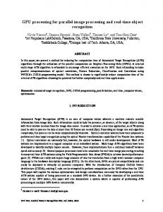
In our cartilage and bone tissue microscopic images, samples are stained with picrosirius or alcian blue to reveal features of either bone (red) or cartilage (blue), for which a single-color histogram suffices (see Figure 1). Other cases like X-ray images or images captured by an electronic microscope work with gray-scale images. For more complex cases where the whole RGB space must be analyzed, the 3D histogram needs to be computed. Such a 3D histogram cannot be derived from the three 1D histograms created above. Both processes share a similar computational load, but the 3D histogram is a task consuming a significantly larger amount of memory (2563 counters space vs. 256 in the 1D case). We implemented it in our hardware as a procedure belonging to the following task. B. Classification into clusters The color-based segmentation is a classification algorithm into regions or clusters based on color affinity [11]. It can be described as a four step process: 1) Compute the 3D RGB color space histogram for each of the biomedical images. 2) Classify into clusters according to an initial guess for the cluster centers in the RGB color space. Iterate to regenerate centers until a convergence criteria is fulfilled. 3) Build the color look-up table (LUT), which maps each 3D color coordinate to the cluster it belongs. 4) Classify each image pixel into clusters according to its colors to obtain the final segmentation. This algorithm has not been previously executed on a GPU. Our starting point is the segmentation process shown in Figure 2.c for a placenta image, which was running in around six minutes on a Laptop computer with a 1.7 GHz Pentium M CPU using Matlab (see [11]). C. Boundary detection Edge detection filters try to identify edges based on gradient magnitudes. Such filters are computed using a convolution mask with different weights in the matrix applied to the adjacent pixels. Operators like Roberts, Prewitt, Sobel and Frei-Chen are defined this way [15]; among all them, we chose the Canny edge detector [5], which is considered the best for a gray-scale or single-color component image. For the cases where the input image covers the whole RGB color space, we start by applying the luminance operator [15] to convert the image from the RGB space to grayscale. Our Canny filter is then followed by a gaussian operator to remove the noise in the image. Finally, edge detetion is processed in two steps: (1) no-maxim removal and (2) hysteresis of double threshold. In the first stage, we set all values to zero that do not represent a local maximum; in the second, we use two threshold values to limit the interval of gray values corresponding to the final boundaries. D. Pattern recognition Techniques for pattern recognition can be classified into two families or clusters depending on local or global processing

1 1 2

2 3

3

(a)

(b)

(c)

Fig. 1. Light microscopy of a segmental defect after 12 weeks of cell implantation. Images are from our biomedical analysis for bone regeneration using stem cells. Samples taken are two consecutive slices at a 7µm thickness. The histochemical staining used is (a) picrosirius-hematoxilin (bone tissue in red) or (b) alcian blue (cartilage in blue). (c) Tissue layers after segmentation: (1) Dense cartilage region, with color center in R=38, G=108 and B=19. (2) Bone tissue, characterized by color center in R=223, G=210 and B=254. (3) Poor cartilage region, with color center in R=140, G=166 and B=236.

(a)

(b)

(c)

Fig. 2. Color image segmentation applied to a 3µ slice for a mouse placenta. (a) Original image. (b) Human validated image. (c) Tissue layers after segmentation: Labyrinth in blue, spongiotropoblast in yellow and glycogen in cyan.

[15]. Among them, we have selected the Hough transform [3], a global technique recognized for its robustness even in the presence of overlap and noise in the image. The Hough transform was recently implemented on GPUs for arbitrary shapes [17]. We restricted our implementation to circular and eliptical shapes, which are of major interest in our biomedical images. This simplifies the computation and presents some GPU benefits as well. Foreground-background segmentation has also been implemented on GPUs with execution times around 4 ms. on a GeForce 6800GT for images of 640x480 pixels [8]. This binary segmentation is not valid for our biomedical purposes, either bone or genetics, where the image size is bigger and regions belong to at least three different entities as explained below. We only take computational time as a cost reference. III. B IOMEDICAL IMAGE PROCESSING A wide variety of histologically stained images in cell biology require deep analysis to determine both the phenotype and color for the tissue being analyzed. One example is cartilage and bone regeneration, where a specific microenvironment has been reported to induce the expression of skeletal matrix proteins, playing a regulatory role in the initiation of cartilage differentiation and the induction of bone-forming

cells from pluripotent mesenchymal stem cells [2] (see Figure 1). Another example is genetics because of the importance of understanding how the genotype (e.g., gene mutations and knockout) affects phenotype (e.g., tissue morphology or animal behaviour) [11]. A solid understanding of the genotypephenotype relationships is valuable in developing therapies to treat diseases related to genotype changes such as cancer. As the genotype change can be well controlled under experimental conditions, it is critical to quantitatively assess the corresponding phenotype change in the organism (see Figure 2). We developed algorithms on the GPU for tracking such biomedical evolution at image level as a preliminary step for converting the complete analysis process to a semi-automatic task: the medical expert interacts with the computer to attain a number of descriptors and attributes about the images that help to understand the biomedical features. The motivation of our work entails a step forward in performance since these algorithms are characterized by a heavy workload and a vast memory use. The current capabilities of GPUs with respect to GFLOPS (arithmetic intensity for a fast computation) and Gbytes/sc (memory bandwidth for a fast data retrieval) are our major keys for a significant reduction in the overall execution time. A. Input data sets The skeletal data set is obtained from implants on 7 month old male rats. After 17 days of culture, in-vivo stem cells are implanted on animals into demineralized bone matrix or diffusion chambers. Four weeks later, rats are sacrificed, six chambers excised and tissues analyzed biochemically or processed for light microscopy after the appropiate fixation and sectioned at 7µm thicknes. From each chamber, approximately 500 slices of tissue sample are obtained, each being a microscopic 1024x1024 RGB color image in TIFF format, for a total storage space of 10 Gbytes. On the other hand, the microscopic images from the genetics working set are obtained from the standard histologically stained slides of both a wildtype and a mutated (Rb-) mouse placenta whose slides are collected by sectioning the wax fixed sample (placenta) at 3µm thickness. They are then digitized using an Aperio Scanscope with a 20x magnification objective lens, producing effective magnification of 200x under which we create images of 20480x20480 pixels, each with a file size between 500 Mbytes and 1 Gbyte. A total of more than 2000 images are obtained (1278 images from the wildtype and 786 images for the Rb-) with an overall file size of 1.7 Terabytes. B. Color analysis Color analysis in our bone regeneration images is related to the staining of the samples, which reveals the histogenic process that is taking place in the induction of cartilage and bone-forming cells from pluripotent mesenchymal stem cells. The shape of the image histogram for each of the red, green and blue color channels deducts key features about tissue regeneration. For example, the red channel is applied when using picrosirius, which reveals bone tissue by the presence

of type I collagen; likewise, the blue channel reveals cartilage tissue by the presence of type II collagen stained with alcian blue (see Figure 1). The 3D histogram is more useful for our genetics applications where it is used as the first step of an image segmentation based on color. C. Phenotype analysis To assess the 3D change of the various tissue types, the first technical step is to segment each image into regions corresponding to the three tissue layers involved depending on the biomedical application: • In the skeletal regeneration example, these layers are represented by cartilage, bone and fibrous tissue. • For the genetic case, these layers are glycogen, labyrinth and spongiotrophoblast. Once this has been accomplished, the serial sections of each image are registered to reconstruct a 3D model of each of the tissue layers by using registration information to align the segmented images. The GPU computer analysis of the phenotype comprises border detection for the tissue using the Canny filter [5] and a subsequent pattern recognition of circular shapes using the Hough transform [3]. An example of application useful in both bone and genetics analysis is to obtain a rough count of the number of cells existing on a particular tissue. IV. I MPLEMENTATION ON THE GPU The extraordinary GPU performance stems from its design simplicity, which enables high parallelism when processing data. The elements in the stream are independent from each other and transformed through unary operators, thus exposing both parallelism and locality while enabling high arithmetic intensity, the ratio of computation to bandwidth. Because the computational power on microprocessors is increasing faster than the communication speed, this results in a very scalable architecture. Overall, the GPU delivers its extraordinary power in computationally demanding algorithms, either because of the heavy data volume or the high number of iterations to process. In this paper, we focus on biomedical applications containing both features, and exploit parallelism at three levels: Instruction, threads and tasks. V. E XPERIMENTAL RESULTS To demonstrate the effectiveness of our techniques, we run our segmentation algorithms on commodity PCs endowed with CPUs from the Pentium family and GPUs from the GeForce series (see Table III). OpenGL 2.0 plus a number of extensions were chosen to map the graphics elements onto the GPU, and the Cg language was selected for programming the vertex and pixel shaders. For the codes on the CPU, we used Visual Studio .NET under Windows XP. Color-based segmentation used the genetic input data set (sections V-A, V-B and V-C) and hardware families 1 and 2 according to Table III, whereas shape-based segmentation used the skeletal data set (sections V-D, V-E and V-F) and hardware family 3.

TABLE I E XECUTION TIMES ON THE HARDWARE FAMILY 1 FOR THE 1D COLOR CHANNEL HISTOGRAM WITH 256 BINS ON A GENETIC 1024 X 1024 TILE .

Code version glHistogram() (computation only) glHistogram() (writing results to frame buffer) glHistogram() (writing results to pixel buffer) occlusion queries (256 renderings) CPU (Pentium 4 540, 3.2 GHz)

Exec. time 140 msc. 3680 msc. 160 msc. 120 msc. 34.4 msc.

TABLE II E XECUTION TIMES ON DIFFERENT PLATFORMS FOR THE COLOR CENTERS COMPUTATION AND THE LOOK - UP TABLE GENERATION ON A GENETIC 1024 X 1024 TILE .

Task to be performed Color centers Look-up table

GeForce 6800 Ultra 904 msc. 40 msc.

GeForce 7800 GTX 155 msc. 20 msc.

Pentium 4 3.2 GHz 850 msc. 1150 msc.

A. 1D and 3D color histograms The 1D histogram is an easy function for implementation on the GPU since OpenGL provides the function glHistogram(). However, the graphics driver in Nvidia cards delegates this computation to the CPU, making it inefficient (see Table I). Because we barely benefit using the GPU for computing the histograms and the expensive GPU-CPU communication cost (see section II-A), the 1D and 3D histograms are delegated to the CPU. This way, we map each computation to the processor that behaves more effectively on it and try to balance the workload on both processors (see Table V). B. Classification into regions The clustering algorithm depicted in section II-B is composed of four steps. After (1) computing the 3D histogram, (2) color centers are calculated to identify each cluster (image region) and weighted by the 3D histogram values, (3) the lookup table (LUT) is built based on minimal distance, and (4) final assignment from colors to regions is done. In the genetics case, due to the massive input data set (see section III-A), it is more efficient to first map 2563 colors to cluster centers using the LUT and then map 2000x20480x20480 pixels to centers using its color as index to the LUT. This is the rationale for building the LUT prior to the final pixel assignment in section V-C. Table II shows the execution numbers for this stage demonstrating the significant impact of the GPU platform, not only with respect to the CPU, but also between different GPU hardware generations. One of the primary reasons for the difference between generations is the higher number of processors in the newest models (see Table III). C. Assign pixels to regions This phase repeats the following sequence until all images have been segmented: Load an image tile and process the segmentation according to LUT. Working on hardware family 2, CPU takes 75 msc. for loading and 11 msc. for processing

TABLE III H ARDWARE FAMILIES USED FOR OUR IMPLEMENTATIONS . T HE G E F ORCE 7950 GX2 IS A DUAL -GPU GRAPHICS CARD WE PROGRAMMED IN A SINGLE -GPU MODE FOR LACK OF UP TO DATE DRIVER SUPPORT.

Hardware family 1 (2004) 2 (2005) 3 (2006) Hardware family 1 (2004) 2 (2005) 3 (2006)

CPU: Pentium 4 model and frequency 540, 3.2 GHz 540, 3.2 GHz D 930, 3 GHz GPU: GeForce model model and frequency 6800Ultra, 425 MHz 7800 GTX, 430 MHz 7950 GX2, 500 MHz

Main memory frequency and size 2x200 MHz & 1 GB. 2x200 MHz & 1 GB. 2x266 MHz & 1 GB. Video memory frequency and size 2x550 MHz & 256 MB. 2x600 MHz & 256 MB. 2x600 MHz & 512 MB.

a single image tile of 1024x1024, whereas GPU spends 6 msc. for loading and 14.2 msc. for processing. Even though the GPU is slower computing, the CPU loading time predominates opening an opportunity for the GPU to help: GPU computation may overlap the CPU loading time for the next image and hide this task. Since the GPU-CPU communication cost is 6 msc, we save 5 msc with respect to the 11 msc. the CPU requires to compute. D. Luminance operator We start our shape analysis by converting biomedical images into grayscale, a step required for further processing. Conversion is performed through the luminance operator [15], which is computed in the pixel processor for the image space. The GPU spends 8.4 msc. for completing this process, which takes as much as 81.3 msc. on the CPU. A 10x improvement factor is achieved on the GPU, even though vector processing cannot be used here on color channels. E. Edge detection: The Canny filter A major challenge for implementing the Canny edge detector on the GPU lies in the quite irregular step of finding and connecting edges to a single object boundary. We have solved this problem by first computing a gaussian distribution for noise removal, followed by the gradient operator in both axis to obtain the final borders before thresholding. Both processes are implemented applying a convolution mask, with an extensive access to textures at the beginning and the presence of simple linear algebra operations in the final part. The combination of data accesses and arithmetic intensity produces the best reward in the GeForce 7950 GX2 given its potential in bandwidth (76 GB/sc.) and processing power (191 GFLOPS). For once, peak hardware ratios are fully exploited by a software operation like the convolution, where the GPU is a renowned masterpiece; otherwise, it would be rather difficult to justify the huge gap opened here between the two processors (see Table IV). F. Pattern recognition: The Hough Transform In most of the GPU implementations, the fragment processor plays the most important role, leaving the vertex processor just for marginal use. However, in our implementation for

TABLE IV E XECUTION TIMES ( IN MILLISECONDS ) ON A CPU AND GPU FOR THE SHAPE SEGMENTATION PROCESS DECOMPOSED IN SUBTASKS ON 1024 X 1024 SKELETAL IMAGE .

Task Luminance Canny Hough

Pentium D 81.3 msc. 1865 msc. 4626 msc.

GeForce 7950 GX2 8.4 msc. 18.6 msc. 980 msc.

Gain 9.67x 100x 4.72x

R EFERENCES

TABLE V S UMMARY OF TASKS DEVELOPED FOR COLOR AND SHAPE SEGMENTATION AND PROCESSOR RESPONSIBLE FOR ITS COMPUTATION . T HE HW COLUMN REFERS TO THE HARDWARE FAMILY OUTLINED IN TABLE III.

C O L O R S H A P E

Task to compute 1D histogram 3D histogram Get color centers Build the 3D LUT Classify pixels Luminance operator Edge detection: Canny filter Pattern recognition: Hough transform

Our results indicate a significant performance improvement for these applications using GPUs versus CPUs of the same generation, reaching factor gains between 4x and 100x depending on the nature of the computations, the hardware family and the programming resources used. We also detected scenarios in which the CPU is faster, showing how both processors can work in parallel for a reduction in the overall execution time.

Input data set Genetics Genetics Genetics Genetics Genetics Skeletal

Winner CPU CPU GPU GPU CPU/GPU GPU

HW 1 2 2 2 2 3

Skeletal

GPU

3

Skeletal

GPU

3

the Hough transform we have achieved a remarkable success exploring this unusual path. Vertex processors are in charge of the evaluation of the analytical expression for the curve, exploiting their skills in transforming positions. However, to obtain the target accumulative space is a tedious task for the GPU. Even though we only pretend to detect circular shapes of a particular radius (matching the cell size), the angle parameter requires to be computed in all its (0, 2π) range, and for each value, we obtain samples that have to be accumulated in the parameters space. To carry this out, we associate the z-position vertex attribute (depth coordinate in the screen geometry) to each angle value. This results in a 3D vertices space where the pixel processor collects data accumulating all values on a single 2D texture. Overall, the vertex processor parametrizes all edges detected for a particular angle value, and the pixel processor uses two textures to perform the accumulation: one of them stores the actual parametrization and the other contains the accumulative space until the current value of the angle. With this implementation, the GPU spends 980 msc. for a 1024x1024 image which contains 35351 vertices coming from the Canny filter. The same process on a CPU spends 4626 msc, that is, a factor of 4.72 worse. Table IV summarizes the times obtained for shape segmentation, and Table V provides the final standings from our work. VI. C ONCLUSIONS We presented a framework for mapping biomedical image analysis onto GPUs, as well as establishing a cooperative environment between the CPU and the GPU. We have applied our techniques to the image segmentation problem, developing color and shape-based algorithms for evaluating GPUs in the genetics and skeletal contexts.

[1] A Web page dedicated to the latest developments in generalpurpose on the GPU. http://www.gpgpu.org. [2] Andrades, J.A., Santamar´ıa, J.A., Nimni, M.E., Becerra, J. Selection, amplification and induction of a bone marrow cell population to the chondro-osteogenic lineage by rhOP-1: an in vitro and in vivo study. International Journal Developmental Biology, vol. 45, pp. 683-693 (2001). [3] Ballard, D. Generalized Hough transform to detect arbitrary patterns. IEEE Trans. on Pattern Analysis and Machine Intel., Vol. 13, no. 2, pp. 111-122, 1981. [4] Beucher, S. The watershed transformation applied to image segmentation. Proceedings 10th Conference on Signal and Image Processing in Microscopy and Microanalysis, pp. 16-19, 1991. [5] Canny, J. A computational approach to edge detection. IEEE Transactions on Pattern Analysis and Machine Intelligence. Vol. 8, no. 6, pp. 679-698, 1986. [6] Fluck, O., Aharon, S., Cremers, D., Rousson, M. GPU Histogram Computation. Poster in Proceedings SIGGRAPH 2006. [7] Govindaraju, N.K., Raghuvanshi, N., Manocha, D. Fast and Approximate Stream Mining of Quantiles and Frequencies Using Graphics Processors. Proceedings SIGMOD 2005. [8] Griesser, A., De Roeck, S., Neubeck, A., Van Gool, L. GPUBased Foreground-Background Segmentation using an Extended Colinearity Criterion. Proceedings VMV 2005, November 1618, Erlangen (Germany). [9] Hadwiger, M., Langer, C., Scharsach, H., Buhler, K. State of the Art Report 2004 on GPU-Based Segmentation. Technical Report TR-VRVis-2004-017. VRVis Research Center, Vienna (Austria). [10] Hendee, W.R. and Ritenour E.R. Medical Imaging Physics. Wiley-Liss, 2002. [11] K. Huang., K. Mosaliganti, T. Pan, J. Saltz. Mouse Placenta: Tissue Layer Segmentation. Procs. 27th Intl. Conf. of the IEEE Engineering in Medicine and Biology Society, 2005. [12] Kass, M., Witkin, A., Terzopoulos, D. Snakes: Active contour models. Intl. Journal of Computer Vision, vol. 1, no. 4, pp. 321331, 1988. [13] Manku, G.S., Motwani, R. Approximate Frequency Counts over Data Streams. 28th VLDB Conf, Hong-Kong (China), 2002. [14] Owens,J.D., Luebke,D., Govindaraju,N., Harris,M., Kruger,J., Lefohn,A.E. and Purcell,T.J. A Survey of General-Purpose Computation on Graphics Hardware. J. Computer Graphics Forum, Vol. 26, No. 1, 2007. [15] Pratt., W.K. Digital Image Processing. John Wiley & Sons, Inc. (1978). ISBN: 0-471-01888-0. [16] Sezgin, M. and Sankur, B. Survey over image thresholding techniques and quantitative performance evaluation. J. Electronic Imaging, vol. 13, no. 1, pp. 146-165, 2004. [17] Strzodka, R. Ihrke, I., Magnor, M. A Graphics Hardware Implementation of the Generalized Hough Transform for fast Object Recognition, Scale and 3D Pose Detection. Int’l Conf. on Image Analysis and Processing, pp. 188-193, 2003. [18] Suri, J., Wu D. A comparison of state-of-the-art diffusion imaging techniques for smoothing medical/non-medical image data. 16th Intl. Conf. on Pattern Recognition, 2006. [19] Weickert, J. A review of nonlinear diffusion filtering. Intl. Conf. on Scale-Space Theory in Computer Vision, pp. 3-28, 1997.