{jethro,huangantâ¡}@fractal.ee.ntu.edu.tw, {phuangâ . ,lei}@cc.ee.ntu.edu.tw. 1. Department of Electrical Engineering. National Taiwan University. 2. Institute of ...
The Impact of Network Variabilities on TCP Clocking Schemes Kuan-Ta Chen12 , Polly Huang1† , Chun-Ying Huang1‡ , and Chin-Laung Lei1 {jethro,huangant‡ }@fractal.ee.ntu.edu.tw, {phuang† ,lei}@cc.ee.ntu.edu.tw 1 Department
of Electrical Engineering National Taiwan University
Abstract— TCP employs a self-clocking scheme that times the sending of packets. In that, the data packets are sent in a burst when the returning acknowledgement packets are received. This self-clocking scheme (also known as ack-clocking) is deemed a key factor to the the burstiness of TCP traffic and the source of various performance problems—high packet loss, long delay, and high delay jitter. Previous work has suggested contradictively the effectiveness of TCP Pacing as a remedy to alleviate the traffic burstiness. In this paper, we analyze systematically and in more robust experiments the impact of network variabilities on the behavior of TCP clocking schemes. We find that 1) aggregated pacing traffic could be burstier than aggregated ack-clocking traffic. Physical explanation and experimental simulations are provided to support this argument. 2) The round-trip time heterogeneity and flow multiplexing significantly influence the behaviors of both ack-clocking and pacing schemes. Evaluating the performance of clocking schemes without considering these effects is prone to inconsistent results. 3) Pacing outperforms ack-clocking in more realistic settings from the traffic burstiness point of view.
I. I NTRODUCTION The idea of packet pacing is not new. The use of this traffic smoothing technique has been introduced in [9] to eliminate the packet bursts caused by ack compression. Aggarwal et. al [2] investigated the performance impacts of packet pacing in TCP. They found that pacing results in lower throughput and higher latency in most of the scenarios they examined. They identified that pacing caused synchronized drops and late congestion signals which are the primary reasons of the performance problem. Motivated by the counter-intuitive results, we set out to evaluate ack-clocking and pacing schemes. In order to understand the underlying mechanism that contribute to the performance problems, we confine our attention to more fundamental behavioral analysis, especially on the analysis of traffic burstiness exhibited by two clocking schemes. We show, in this paper, that aggregated pacing traffic could be burstier than aggregated ack-clocking traffic. This finding is supported by the behavioral models of the two clocking schemes and simulation results. In addition, we observe that the behavior of the two clocking schemes could be very different depending on the network conditions. This suggests that it is critical in performance evaluation of the two schemes to experiment on network settings of sufficient variabilities. The comparative traffic burstiness of TCP ack-clocking and pacing are largely affected
2 Institute
of Information Science Academia Sinica
by the two factors— 1) whether the round-trip times (RTT) of aggregated flows are the same or not, and 2) the number of flows participated at the bottleneck. Our observations echo the results in [2] since most of their simulation scenarios are configured as homogeneous RTT and pacing tends to be burstier than ack-clocking in such conditions. However, in a more realistic settings with heterogeneous RTT and/or other forms of variability, pacing is always less bursty than ackclocking according to our analysis. The remainder of the paper discuss these issues in more details. In Section II, we discuss previous work in this area. Section III describes the methodology concerning traffic burstiness estimate. In Section IV, we provide two behavioral models to illustrate why pacing could be burstier in certain conditions. In Section V, we conduct network simulations to validate the behavioral models and explore the impact of various network variabilities on respective clocking schemes. Finally we conclude in Section VI. II. R ELATED W ORK Pacing is a clocking scheme which combines the characteristics of rate control and window control, that is, the release of packets are scheduled by timers with the limit of window size. Since [9] initially introduced pacing to adjust the incorrect timing from ack compression, other researchers have suggested using the concept of pacing in various circumstances; for example, to avoid slow start at start-up of a connection [6], or avoid bursts when an idle connection resumes [10]. Partridge [7] argues that pacing can alleviate the problems in TCP performance on long latency and high bandwidth satellite links. Razdan [8] proposed enhancements combining TCP Westwood [11] and packet pacing to improve TCP performance with small buffers. Though the concept of pacing has been used in many ways, however, few attempts have been made on the analysis and evaluation of pacing. Among these, [2] was one of the first work on the performance evaluation of TCP Pacing. The paper shows that pacing often results in lower throughput and higher latencies. While the subject of this paper overlaps significantly with [2], our work differs in two ways: 1) This paper emphasizes the behavioral analysis rather than the performance comparison of clocking schemes. 2) We focus on how the
round trip time T
τ
(a) ack-clocking
(b) pacing
round trip time T
(T-18τ)/3
τ
(a) ack-clocking
T/6
T/18
flow 1
flow 2
(T-18τ)/3
flow 3
Fig. 1. Packet arrival patterns in our models. Each flow has equal window size of six.
network variability affects the traffic burstiness of clocking schemes. III. M ETHODOLOGY To evaluate TCP clocking schemes, we focus on analyzing the level of burstiness in the traffic since traffic burstiness is an indicator of performance, especially for delay and drops. In this paper, we shall concentrate on behavioral analysis in terms of traffic burstiness measure. With respect to burstiness estimation, we use the method wavelet-based MultiResolution Analysis [1] to analyze the burstiness of a traffic process over a range of time scales. The traffic process in a network can be described as a time series of packets or bytes arrived. It is commonly used that a traffic process is defined as a counting process {Xj } = {Xj,0 , Xj,1 , . . .} at a time scale Tj = 2j T0 where T0 is called the reference time scale. The term “burstiness” refers to the statistical variability at a certain time scale Tj . In this paper the burstiness is defined as the variance of the Haar wavelet coefficients at a given scale [5], and it is also known as the energy. The Haar wavelet coefficients Wj,k at time scale Tj are defined as Wj,k = 2−j/2 (Xj−1,2k − Xj−1,2k+1 ). The energy εj at time scale Tj is then computed by the variance of time series {Wj } as εj = V ar(Wj ) = 2−j E[(∆Xj−1,k )2 ] where ∆Xj−1,k is defined as (Xj−1,2k − Xj−1,2k+1 ) and E[∆Xj−1,k ] = 0 is assumed. In practice, the energy εj is estimated from a finte time series as �Nj 2 −j k=1 (∆Xj−1,k ) εj ≈ 2 Nj where Nj is the number of wavelet coefficients at scale j. We use the energy plots for level of burstiness observations. An energy plot shows the energy of the traffic process {Xj } as a function of time scale Tj . To put it concretely, we count the total bytes arrived at the selected bottleneck link every T0 = 0.1 ms to obtain the time series {X0 }, which is used to compute the energy ε1 at time scale T1 = 20 T0 = 0.1 ms. We can then calculate time series in larger scales by aggregation. The aggregation means smoothing the original time series {X0 } by averaging the observations over nonoverlapping blocks of size 2j to get a new time series {Xj }.
(b) pacing
T/5
flow 1
flow 2
flow 3
T/10
back-to-back
Fig. 2. Packet arrival patterns with unsynchronized windows. The packets of different flows occasionally collide with each other, and form back-to-back packet bursts at the bottleneck.
Since we concentrate on sub-RTT behaviors in this paper, we are only interested in time scales up to a half RTT. An example of energy plots is shown in Fig. 5(a). Note that the top x-axis of the figure displays Tj−1 in mini-seconds while the bottom x-axis shows j, since the energy εi is determined by ∆Xj−1,k at previous scale Tj−1 . To understand the behaviors of clocking schemes, generally we observe the burstiness discrepancy exhibited by different clocking schemes at various time scales. Occasionally we shall contrast the traffic burstiness with that of a Poisson process to reveal the relative burstiness of our TCP traffic between an independent inter-arrival counting process. IV. W HY PACING C OULD BE B URSTIER ? Intuitively, even we do not know whether pacing yields better performance yet, pacing should be less bursty than ackclocking, or be at equal burstiness in the minimum case. In this section, we describe why pacing could become burstier than ack-clocking in certain cases, and we shall show how this behavior can be eliminated in the next section. A. Behavioral Models For the illustration of the counter-intuitive phenomenon, two behavioral models are provided: one is for ack-clocking, and another is for pacing. To capture the essence of traffic pattern exhibited by ack-clocking flows, we make use of the packettrain model proposed by Chiu and Jain [4]: for a flow with window w, in a round-trip time T , the model will release w packets spaced at a constant interval τ0 while keeping idle in the remaining time (T − wτ0 ). In our model, the interval τ0 is set to the packet service time at bottleneck link τ = L/B, where L denotes packet size and B is the bottleneck link bandwidth. For N > 1 aggregated flows, where flow i has window size wi , the inter-packet-train � time between different flows is computed by ts = (T − τ wi )/N . After that, we can schedule each flow’s packet-train sequentially with spacing ts , as shown in Fig. 1(a). In the pacing behavioral model, w packets are completely spread out in a round-trip time T with inter-spacing ∆ = T /w. When N flows are aggregated, the packets from different flows are mixed, and the inter-packet time is set to T /(N · w). In the case window sizes are not synchronized, the spacing time of each flow’s first packet is set to T /(N · max(wi )) to avoid packets from different flows colliding with each other.
S1 0.2 18
16
0.4
0.8
3.2
12.8
51.2
3 ack-clocking (30,30,30) 3 ack-clocking (20,30,40) 3 pacing (30,30,30) 3 pacing (20,30,40)
Bs
x Mbps (bottleneck)
BR 4x Mbps
14 log2(energy)
R1
4x Mbps
102.4 (ms)
SN
12
RN
(a) Dumbbell topology
10
4x Mbps
8
R1
6
x Mbps
R2
R3
R4
R11
4 2
4
6 log2(scale)
8
10
11
Fig. 3. The impact of window un-synchronization effect. Window unsynchronization makes pacing burstier, while the same effect does not affect the burstiness of ack-clocking.
Fig. 1 illustrates the packet arrival patterns for three flows according to the above behavioral models, where each flow has equal window size of six. With ack-clocking, the six packets of each flow are sent in burst with silence in the next 4τ , and then the next flow sets out. The packets from the same flow are clustered together. On the contrary, in the pacing model, packets are sent evenly within a round-trip time, and the packets from different flows are mixed. B. Window Un-Synchronization Effect Though the packets arranged by pacing are sent out evenly in Fig. 1, but in reality, the property of even spacing may not exist since window sizes of different flows are usually unsynchronized. In Fig. 2, we show the packet arrival patterns of three flows with different window size 5, 3, and 10, respectively. To ack-clocking, unsynchronized windows just affects the relative time of packet-trains, but at the same time, unsynchronized windows leads to uneven spacing of packets with the pacing scheme. Occasionally the packets of different flows are arrived the bottleneck back-to-back where we annotate the packets with an explosion mark. Our observation is that window un-synchronization makes pacing burstier, while the same effect does not affect the burstiness of ack-clocking. To quantitatively judge the impact of window un-synchronization effect on traffic burstiness, we assess the burstiness for synthesized traffic which is generated by the behavioral models. To keep it simple and clear, we assume a scenario with T = 100 ms and τ = 0.1 ms; three flows are running, where their window sizes are set to (30, 30, 30) and (20, 30, 40), respectively. The measured traffic burstiness for both schemes with and without window unsynchronization is shown in Fig. 3. In the graph, we can see that ack-clocking traffic only raises its burstiness a bit at scale RTT/4 with the effect of window un-synchronization. It follows that the packets distributes more unevenly in different quarters of RTT, but the traffic variability at finer scales keeps untouched. On the other hand, pacing suffers significant burstiness increase at nearly all time scales. The explanation
(b) Parking-lot topology Fig. 4.
The network topology used in simulations.
is obvious from Fig. 2 since the periodic structure of pacing has been destroyed by the unsynchronized window sizes. Furthermore, the abrupt packet bursts can cause unnecessary queueing and packet drops. In practice, since window size is continuously changing during the whole lifetime of a connection, the inter-packet spacing ∆ for paced packets is varied as well. As more randomized the inter-packet time and more multiplexing flows at the bottleneck, the tendency of paced packets from different flows colliding with each other is stronger. By simulations, what we shall show in the next section, as more flows are aggregated, the traffic burstiness of pacing could become burstier than ack-clocking in most of sub-RTT time scales. V. S IMULATIONS In this section, packet-level network simulations are conducted to verify the observations in Section IV and to examine the impact of different network variabilities on TCP clocking schemes. After defining the simulation setup, we investigate the impact of flow multiplexing, RTT heterogeneity, and other variabilities in sequence. We shall show flow multiplexing and RTT heterogeneity are two deciding factors on the behaviors of TCP clocking schemes. A. Setup We use the network simulator ns-2 [3] to perform simulations in this paper. Fig. 4(a) shows the dumbbell topology used in most simulations. In that, a single bottleneck link with bandwidth x Mbps is set. A TCP flow fi is established between each pair of hosts Si and Ri . FIFO scheduling and drop-tail queueing discipline is used. The bottleneck queue size is calculated in terms of bandwidth-delay product (BDP); it is defined in packets and assigned to 25% of BDP. The links connecting hosts and routers are provided with theoretic infinite buffer size to avoid being bottlenecks. Similarly, the maximum advertised window for TCP connections is set to a high enough value so that the congestion window is
0.2
0.4
0.8
3.2
12.8
51.2
102.4 (ms)
0.2
0.4
0.8
3.2
12.8
51.2
102.4 (ms)
0.2
26
22
22
20
24 22
0.8
3.2
12.8
51.2
102.4 (ms)
log2(energy)
18
16
16
14
14
12
12
10
10
8
8
10
11
ack-clocking 1 flow pacing 1 flow ack-clocking 50 flows pacing 50 flows Poisson
20
18
20 log2(energy)
1 flow 2 flows 5 flows 50 flows Poisson
log2(energy)
24
0.4
26 1 flow 2 flows 5 flows 50 flows Poisson
18 16 14 12
8
10 8
6 2
4
6 log2(scale)
8
10
11
6 2
4
6 log2(scale)
8
10
11
(a) Ack-clocking: The burstiness of ack-clocking (b) Pacing: The burstiness of pacing traffic traffic tends to approach Poisson as more flows become higher as more flows are involved. are involved. Fig. 5.
2
4
6 log2(scale)
(c) A single flow vs. 50 flows aggregated. With a single flow, ack-clocking is much burstier, however, ack-clocking and pacing become comparable when 50 flows are involved.
Traffic burstiness evolution on the effect of flow multiplexing. Homogeneous RTT is assumed.
not limited. We use packet size of 576 bytes. Fig. 4(b) is the parking lot topology used in Section V-D, and we defer the description of the network topology to that section. The simulation duration is fixed to 200 seconds. Since we concentrate on the behaviors of clocking schemes rather than TCP congestion control, the traffic during the first 20 second is simply discarded to keep away from the effect of TCP’s slow start mechanism. We use TCP Reno as our “test bed” of clocking schemes. Other TCP variants such as TCP Tahoe should lead to similar results since clocking schemes control the behaviors within a round-trip time while TCP variants primarily differ in window control mechanisms. The Reno code in ns-2 [3] is taken as the implementation of ack-clocking scheme, and the pacing scheme is modified based on the same code. In our implementation of TCP Pacing, every time a packet is sent, a pacing timer schedules a timeout of interval ∆ = RT T /w. No new packets could be sent before the timer expires. Whenever the pacing timer expires, exactly one packet could be sent if one or more packets are awaiting, and another timeout is scheduled if needed. The timeout interval is re-computed each time when the pacing timer is to be scheduled.
is much lower than the single flow case and is even lower than Poisson. The behavior shows that in homogeneous RTT scenarios, the bursty nature of TCP ack-clocking could be reduced by aggregation. In contrast, flow multiplexing has much different influence on pacing. With a single flow, pacing exhibits low traffic burstiness across sub-RTT scales. The reason is clear since pacing is actually a periodic process with interval RT T /w. Nevertheless, because of the window un-synchronization effect, the traffic burstiness of pacing raises very quickly as more flows are added, even the join of the second flow brings in considerable influence. In the case that 50 flows are aggregated, as shown in Fig. 5(b), the small scale burstiness approaches Poisson. In other words, the periodic structure has been almost completely broken due to multiplexing. Fig. 5(c) compares the traffic burstiness of both clocking schemes side-by-side. It can be seen that: 1) when 50 flows are aggregated, pacing is burstier than ack-clocking in most sub-RTT time scales, and 2) the comparative burstiness of the two schemes are drastically different with and without flow multiplexing. The phenomenon manifests the importance of level of aggregation on evaluating clocking schemes.
B. The Effect of Multiplexing
C. The Effect of RTT Heterogeneity
In Section IV-B, we have shown that the uneven spacing of paced packets makes traffic burstier. A series of simulations is conducted to show that the effect of window unsynchronization could be amplified by flow multiplexing, and consequently pacing could become burstier than ack-clocking in homogeneous RTT scenarios. To demonstrate, we set the RTT of all flows to 100 ms and vary the flow count from 1 to 50 to examine the variation in traffic burstiness. Fig. 5(a) and Fig. 5(b) show the burstiness variation at different level of aggregation. We first discuss the behavior of ack-clocking. As intuition, when few flows are aggregated, ack-clocking is much burstier than pacing, however, as more flows are involved, the burstiness at small scales slowly increases, and the burstiness at large scales quickly declines. In the case of 50 flows, the small scale burstiness is raised but still less than that of Poisson; the large scale burstiness
In realistic networks, flows along the same path do not necessarily share the same round-trip time. We shall explore the effect of RTT heterogeneity on the behaviors of clocking schemes in this section. The simulation setup is similar to Section V-B except for the choice of flow RTT: instead of using a fixed value of 100 ms, now the value is drawn from an uniform distribution over 100 ms through 300 ms. The results show that heterogeneous RTT makes multiplexed ack-clocking flows much burstier than homogeneous RTT; the burstiness trend in the two scenarios are marked as “Fixed” and “VarRTT” respectively in Fig. 6(a). We find that: 1) the high variability in large time scales comes from the mismatch of RTT, since flows with diverse RTT distribute their packet-trains unevenly. 2) Since the transmission time between each sender and bottleneck link are usually different, the ack-solicited packets are no longer ideally spaced by τ
0.2
0.4
0.8
3.2
12.8
51.2
102.4 (ms)
0.2
0.4
0.8
3.2
12.8
51.2
102.4 (ms)
8
10
11
22
20
18
Fixed VarRTT TwoWay TwoWay* (VarRTT) Cross Real Poisson
14
log2(energy)
log2(energy)
12
16
14
10
12
10
8 2
4
6 log2(scale)
8
10
11
(a) Ack-clocking: all scenarios with heterogeneous RTT behaves approximately the same. Fig. 6.
Fixed VarRTT TwoWay TwoWay* (VarRTT) Cross Real Poisson 2
4
6 log2(scale)
(b) Pacing is resistant to network variabilities. Traffic burstiness in all scenarios are approximately the same.
The traffic burstiness of ack-cloking and pacing traffic, under scenarios with various network variabilities. The trend name is coded by Table I.
(the bottleneck packet service time), but instead governed by the relative length of RTT. When flow number is considerable and/or RTTs are diverse enough, the small scale burstiness of aggregate traffic tends to approach Poisson. In contrast to ack-clocking, the diversity of RTT does not affect pacing, as shown in Fig. 6(b). The main reason is the heterogeneity in RTT and that in window size have exactly the same effect—they bring the randomness of pacing interval ∆ = RT T /w. Since pacing interval is already randomized by of window un-synchronization, RTT heterogeneity cannot induce additional influence. Therefore we can summarize that the heterogeneity of RTT makes ack-clocking traffic burstier, however, the same effect does not exist for pacing traffic. D. More Network Variabilities To further inspect the effects of other network variabilities, we have conducted more simulations, based on the same setup in Section V-B, with additional types of network variabilities or their combinations considered. Specifically, we considered the effects of multi-hop, cross-traffic, and two-way traffic, as listed in Table I. The additional simulation setup is summarized as follows: 1) all simulations in this section are running with 50 flows, i.e., the effect of multiplexing is not examined again. 2) The cross-traffic is provided by putting randomly chosen 10–30 UDP flows at each “backbone” link; the traffic generation is according to Pareto-distributed ON/OFF periods with shape 1.5; packet size is randomly chosen within 100 to 300 bytes; the total cross-traffic rate is adjusted to half of the link bandwidth. 3) Two-way traffic are achieved by exchanging the locations of senders and receivers for half flows. 4) For multi-hop scenarios, we provided a parking-lot topology as depicted in Fig. 4(b): the network has 10 “backbone” links connected by 11 routers; each link has different propagation delays, and each flow has randomly chosen 1–10 hops distance with randomly chosen sender and receiver locations. Fig. 6 shows the traffic burstiness exhibited by two clocking schemes with different combinations of network variabilities. To ack-clocking scheme, it can been seen that the four heterogeneous RTT scenarios share similar traffic burstiness
TABLE I N ETWORK VARIABILITIES S IMULATION S CENARIOS ID Fixed VarRTT TwoWay TwoWay* Cross Real
Topology Dumbell Dumbell Dumbell Dumbell Dumbell Parking-lot
RTT heterogeneity √ √ √ √
Two-way traffic √ √ √
Cross traffic √ √
where two homogenous RTT scenarios present much different behaviors. On the other hand, none of network variabilities significantly affects pacing’s behavior. In addition, the plot reveals an attractive property of pacing, that is, the more randomness (especially two-way traffic), the lower its traffic burstiness. Based on the burstiness plot of Poisson process in Fig. 6, the comparative traffic burstiness of two clocking schemes is clear. In all heterogeneous RTT scenarios, the burstiness of ack-clocking is no lower than Poisson, however, that of pacing is not higher than Poisson across sub-RTT time scales. In brief, pacing is less bursty than ack-clocking as long as flows RTT are heterogeneous. VI. C ONCLUSIONS The observation that “aggregate pacing traffic could be burstier than aggregate ack-clocking traffic” seems counterintuitive at the first glance. In this paper, we have provided physical explanation for the phenomenon by behavioral models, and have also validated the models by experimental simulations. We have shown the behaviors of the two TCP clocking schemes, ack-clocking and pacing, are network condition dependent. The RTT heterogeneity and flow multiplexing are especially critical factors. In general, pacing would exhibit lower burstiness, which implies lower queueing delay and loss, with more network variabilities. Therefore, it is critical that in performance evaluation of these clocking schemes, to experiment with network settings of sufficient variabilities.
R EFERENCES [1] P. Abry and D. Veitch, “Wavelet analysis of long-rangedependent traffic,” IEEE Trans. Information Theory, vol. 44, no. 1, pp. 2–15, Jan 1998. [2] A. Aggarwal, S. Savage, and T. Anderson, “Understanding the performance of TCP pacing,” in INFOCOM (3), 2000, pp. 1157–1165. [Online]. Available: citeseer.nj.nec.com/aggarwal00understanding.html [3] L. Breslau, D. Estrin, K. Fall, S. Floyd, J. Heidemann, A. Helmy, P. Huang, S. McCanne, K. Varadhan, Y. Xu, and H. Yu, “Advances in network simulation,” IEEE Computer, vol. 33, no. 5, pp. 59–67, 2000. [4] D. M. Chiu and R. Jain, “Analysis of the increase and decrease algorithms for congestion avoidance in computer networks,” Comput. Netw. ISDN Syst., vol. 17, no. 1, pp. 1–14, 1989. [5] H. Jiang and C. Dovrolis, “The origin of TCP traffic burstiness in short time scales, Tech. Rep. GIT-CERCS04-09, 2004. [6] V. Padmanabhan and R. Katz, “TCP fast start: a technique for speeding up web transfers,” in Proceedings of IEEE GLOBECOM’98, Sydney, Australia, 1998, pp. 41–46. [Online]. Available: citeseer.ist.psu.edu/padmanabhan98tcp.html [7] C. Partridge, “ACK spacing for high bandwidthdelay paths with insufficient buffering,” Work in Progress, Internet Draft. 1998. [Online]. Available: citeseer.ist.psu.edu/padmanabhan98tcp.html [8] A. Razdan, A. Nandan, R. Wang, M. Y. Sanadidi, and M. Gerla, “Enhancing TCP performance in networks with small buffers,” in Proceedings of Eleventh International Conference on Computer Communications and Networks, 2002, pp. 39–44. [9] S. Shenker, L. Zhang, and D. Clark, “Some observations on the dynamics of a congestion control algorithm,” ACM Computer Communication Review, pp. 30–39, 1990. [Online]. Available: citeseer.ist.psu.edu/shenker90some.html [10] V. Visweswaraiah and J. Heidemann, “Improving restart of idle TCP connections,” Technical Report 97-661, University of Southern California, Nov. 1997. [Online]. Available: citeseer.ist.psu.edu/visweswaraiah97improving.html [11] A. Zanella, G. Procissi, M. Gerla, and M. Sanadidi, “TCP westwood: Analytic model and performance evaluation,” in Proceedings of IEEE Globecom, 2001, pp. 1703–1707. [Online]. Available: citeseer.ist.psu.edu/zanella01tcp.html