The Impact of Preprocessing on Support Vector ... - CiteSeerX

The Impact of Preprocessing on Support Vector Regression and Neural Networks in Time Series Prediction Sven F. Crone, Jose Guajardo, and Richard Weber 27]

Abstract— Support Vector Regression (SVR) and Neural Networks (NN) have been successfully applied to forecasting and time series prediction. While conventional statistical methods require specific data preprocessing prior to the forecasting step both, SVR as well as NN need less efforts for the respective tasks due to their theoretical properties. On the other hand, it is known that preprocessing affects performance of classifiers built using these methods. In this paper we analyze how preprocessing affects the forecasting performance using SVR and NN and provide detailed insights applying several preprocessing strategies to different artificial time series. There is evidence to prefer linear scaling into the interval [-0.5,0.5] among the analyzed strategies. Future work is proposed in order to validate our findings and extend the experiments to alternative preprocessing strategies.

S

I. INTRODUCTION

upport vector regression (SVR) and artificial neural networks (NN) have found increasing consideration in forecasting theory, leading to applications in time series prediction and explanatory forecasting in various domains, including business and management science [1, 2]. In specific cases, these Computational Intelligence methods could show their advantages outperforming conventional statistical approaches such as ARIMA and exponential smoothing; see e.g. [3, 26]. Despite their theoretical capabilities and successful applications, NN as well as SVR are not yet established forecasting methods in business practice. Recently, substantial theoretical criticism towards NN has raised doubts as to their ability to forecast even simple time series patterns of seasonality or trends without adequate data preprocessing [3]. NN and SVR offer many degrees of freedom in the modelling process through the selection of activation or kernel functions and their parameters etc. as well as the stages preceding the model building through alternative forms of preprocessing. It has been shown that data preprocessing is a crucial step in many data mining applications where data cleansing and transformation are applied in order to improve the respective results; see e.g. [25]. Consequently, NN and This work was supported in part by the Millennium Nucleus “Complex Engineering Systems” (www.sistemasdeingenieria.cl) and the Chilean project Fondecyt 1040926. Sven F. Crone is with the Department of Management Science, Lancaster University Management School, Lancaster LA1 4YX, United Kingdom (corresponding author, phone: +44.1524.5-92991, e-mail: [email protected]). Jose Guajardo, Richard Weber are with the Department of Industrial Engineering, University of Chile, Republica 701, Santiago, Chile (e-mail: {jguajard,rweber}@dii.uchile.cl,).

Support Vector Machines (SVM) must be considered sensitive to scale and magnitude of the presented data and therefore to the form of data preprocessing. Consequently, well-defined methodologies including appropriate preprocessing strategies have been developed and applied for clustering [20, 21, 23] and classification tasks [11, 28]. For example, Graf et al. show that the type of preprocessing is an important issue in clustering; see e.g. [23], where 7 different preprocessing strategies have been evaluated, obtaining that linear scaling in the interval [0;1] is one of the two strategies which lead to the most relevant improvements in the cluster structures found. Crone et al. analyse the importance of different forms of data preprocessing on classification accuracy and conclude that preprocessing choices have a stronger impact on accuracy then model building or parameterization of NN, SVM and decision trees [27]. Therefore a structured evaluation of the impact of data pre-processing on the accuracy of methods from computational intelligence is also required for applications in regression tasks of time series forecasting. This paper contributes to the mentioned problems, presenting an analysis of different preprocessing strategies in the form of an empirical simulation experiment of different artificial, archetypical time series. More specifically, we evaluate normalization and linear scaling applied to various time series. Our findings provide insights on usability and limitations of the strategies analyzed. This paper is organized as follows. First, we briefly introduce SVR and NN for the context of time series forecasting. Section III presents the experimental design and the results obtained. Finally, we provide conclusions and future work in section IV.

II. MODELLING SVR AND NN FOR FORECASTING A. Support Vector Regression We briefly describe the standard Support Vector Regression (SVR) algorithm, which uses the ε-insensitive loss function, proposed by Vapnik [5]. This function allows a tolerance degree to errors not greater than ε. The description is based on the terminology used in [6, 7]. Let {(x1,y1),….., (xℓ,yℓ)}, where xi є Rn and yi є R, be the training data points available to build a regression model. The SVR algorithm applies a transformation function Φ to the original data points from the initial Input Space, to

a generally higher-dimensional Feature Space F. In this new space, we construct a linear model, which corresponds to a non-linear model in the original space:

Φ : Rn → F, w ∈ F

(1)

f ( x) = w, Φ ( x) + b

(2)

The goal when using the ε-insensitive loss function is to find a function that fits current training data with a deviation less or equal to ε, and at the same time is as flat as possible. This means that one seeks for a small weight vector w; one way to do that is e.g. by minimizing the quadratic norm of the vector w [6]. As this problem could be infeasible, slack variables ξi, ξi* are introduced to allow error levels greater than ε, arriving to the formulation proposed in [5]:

Min

A 1 2 w + C ∑ (ξ i + ξ i* ) 2 i =1

s.t. y i − w, Φ ( xi ) − b ≤ ε + ξ i w, Φ ( xi ) + b − y i ≤ ε + ξ

(3)

* i

ξ i , ξ i* ≥ 0, i = 1,2,..., A This is known as the primal problem of the SVR algorithm. The objective function takes into account generalization ability and accuracy in the training set, and embodies the structural risk minimization principle [8]. Parameter C measures the trade-off between generalization ability and accuracy in the training data, and parameter ε defines the degree of tolerance to errors. To solve the problem stated above, it is more convenient to represent the problem in its dual form. For this purpose, a Lagrange function is constructed, and in applying saddle point conditions it can be shown that the following solution is obtained [8]: A

w = ∑ (α i − α i* )Φ ( xi )

(4)

i =1

A

f ( x) = ∑ (α i − α ) K ( xi , x) − b i =1

* i

(5)

Here, αi and αi* are the dual variables, and the expression K(xi,x) represents the inner product between Φ(xi) and Φ(x), which is known as the kernel function [8]. The existence of such a function allows us to obtain a solution for the original regression problem, without considering explicitly the transformation Φ(x) applied to the data. In our experiments we use RBF and linear kernel functions. It is well known that when dealing with SVM in classification problems, normalizing input data can heavily influence on the respective results [22]. As stated in [18], normalization is required for particular kernels

due to their restrictive domain (e.g. B splines), and can also be helpful for unrestricted kernels, avoiding problems with the Hessian in the optimization problem. In [19] it has been shown that the type of normalization carried out has an important influence in SVM model performance in the case of classification; moreover, it has been suggested to normalize data in the feature space (not the input space) when training a SVM. In the same sense, [21, 22] point out that the application of normalization techniques in the input space may cause scale problems in the feature space; to deal with this problem, they propose normalizing the kernel function instead of normalizing the original input vectors (in the case of monomial kernels both strategies are equivalent), which leads to a modified SVM algorithm. By using this novel normalization strategy they outperformed a traditional normalization procedure in some pattern recognition problems. Some experiments have shown that the use of polynomial kernels functions without normalization, could lead to overfitting problems when the degree of the function is too large [5]. Finally, [24] suggest to conduct simple scaling on the data to the interval [0,1] or [-1,1] as a previous step when using SVM for classification. However, little information is published on the effects of preprocessing on the performance of SVR in regression tasks. B. Neural Networks Forecasting with non-recurrent NNs requires the prediction of a dependent variable from lagged realizations of the predictor variable, explanatory variables of metric, ordinal or nominal scale and/or lagged realizations thereof. Therefore, NNs offer many degrees of freedom in the forecasting design, permitting explanatory or causal forecasting through estimation of a functional relationship, as well as general transfer function models and simple time series prediction. Next, we analyze briefly the degrees of freedom in modelling artificial NNs for time series prediction; a general discussion is given in [11, 13]. Forecasting time series with NN is frequently modelled in analogy to a non-linear autoregressive AR(p) model [2, 14]. At a point in time t, a one-step ahead forecast is computed using p=n observations from n preceding points in time t, t-1, t-2, …, t-n+1, with n denoting the number of input units of the NN. This models a time series prediction as of

yˆt +1 = f ( yt , yt −1 ,..., yt − n +1 )

(6)

Data is presented to the MLP as a sliding window over the time series observations. The task of the MLP is to model the underlying generator of the data during training, so that a valid forecast is made when the trained NN network is subsequently presented with a new input vector value. The general architecture of a feed-forward Multilayer Perceptron (MLP) is displayed in figure 1.

200 150 100 50 0

yˆt +1

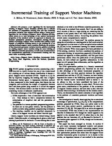
methods we create a set of benchmark time series for the most common time series patterns: linear trend and different forms of seasonality. Consequently, we create individual time series patterns and combine them accordingly, overlaying each with additive noise. As an increasing seasonality along time to reflect a multiplicative seasonality L*SM+E seemed of little empirical relevance in the absence of level changes, it was omitted from further analysis. No Additive Multiplicative Seasonality (E) Seasonality (SA) Seasonality (SM)

yˆt + 2

yˆt + h

No Trend Fig. 1. Autoregressive MLP application to time series forecasting using n input neurons for observations in t, t-1, t-2, …, t-n-1, m hidden units, h output units for time periods t+1, t+2, …, t+h and two layers of trainable weights. The bias node is not displayed.

The network paradigm of MLP offers extensive degrees of freedom in modelling for prediction tasks. Structuring the degrees of freedom, each expert must decide upon the selection and sampling of datasets, the degrees of data preprocessing, the static architectural properties, the signal processing within nodes and the learning algorithm in order to achieve the design goal, characterized through the objective function or error function. For a detailed discussion of these issues and the ability of NN to forecast univariate time series, the reader is referred to [2]. Data preprocessing of the input vector is considered a mandatry requirement for the application of MLPs [28, 29]. As the sigmoid activation functions in the hidden nodes are only defined in the interval of ]-1, 1[ for the hyperbolic tangent or ]0, 1[ for the logistic function, input data must be scaled to facilitate learning [12]. Tang and Fishwick recommend linear scaling data in to smaller intervals, e.g. [0.2, 0.8], to avoid saturation effects at the asymptoic bounds of the activation functions [30]. Consequently, alternative scalings will be considered in our evaluation.

III. EXPERIMENTAL DESIGN

AND RESULTS

A. Description of the Artificial Time Series We evaluate a set of five artificial time series of monthly retail sales motivated from Pegel’s original classification, later extended by Gardner to incorporate degressive trends. Time series are composed of regular patterns of different forms of linear, progressive, degressive or regressive trends T, additively or multiplicatively combined with seasonality S, a constant level L and residual noise E. In addition, empirical time series are impacted by irregular patterns such as level shifts and pulses, which are disregarded in this paper. To evaluate the ability of different computational intelligence

Linear Trend (TL)

Fig. 2. Basic time series patterns of artificial time series according to the Pegels- and Gardner-classification, combining Level, Trend and Seasonality with a medium additive noise level.

Consequently, we create a set of five time series including a stationary time series L+E (E), seasonality without trend L+SA+E (SA), linear trend L+TL+E (TL), linear trend with additive seasonality L+TL+SA+E (TLSA) and linear trend with multiplicative seasonality depending on the level of the time series L+TL*SM+E (TLSM). The residual error term follows a Gaussian distribution N(0,σ2) applying a moderate level of noise σ2=25. The original time series data was taken from the experiments performed in [3] and represent monthly retail sales. All time series consider additive noise terms to allow an estimation of final forecasting accuracy in relation to the original noise level. Each time series consists of 228 observations. B. Experimental Design To scale time series data into adequate intervals for NN and SVR, both linear scaling and normalization, can be applied. Linear scaling transforms the observations into a predefined interval, e.g. [0, 1], [-1, 1], scaling the data into an arbitrary interval defined by a lower bound lb and an upper bound ub, [lb, ub]. The observations Xi of a variable X are transformed according to:

Z i = lb +

X i − MIN ( X ) *(ub − lb) MAX ( X ) − MIN ( X )

(8)

However, linear scaling is sensitive to extreme values and outliers, as the observations may be dominated by a single large value. As an alternative to linear scaling, normalization, also known as z-score normalization, zeromean normalization or standardisation is a scaling

procedure based on the mean and the standard deviation (SD) of a variable. Given a variable X, the following transformation is applied to each observation Xi:

for Poly SVR we set the degree equal to 2 and apply the same scheme.

X − mean( X ) Zi = i SD( X )

For NN models, we used the backpropagation algorithm to construct multi- layer perceptron networks. Models were initialized 20 times using an (13-8-1) architecture comprised of 13 input nodes, 8 hidden nodes and a single output node for t+1 predictions, applying a sigmoid transfer function between the input and hidden layers, and a linear function between hidden and output layers. As for SVR models, we selected the network with the lowest mean absolute error (MAE) on the validation set to calculate the test error results. For more details the reader is referred to [16].

(7)

After scaling, all variables follow a normal distribution with zero mean. However, observations scaled using a normalization procedure will not fall within the interval of [-1, 1] depending on the distribution of the observations. Both, normalization and linear scaling procedures involve aggregated calculations (mean, maximum, etc) based only on in-sample data, i.e. training and validation sets; test set data points are not taken into account to calculate such measures, which implies that in linear scaling these data points could lay out of the bounds of the [lb, ub] interval once they are transformed. Once the predictive model is developed using scaled data, inverse transformation are carried out to obtain final predictions. In this paper we examine 3 different preprocessing strategies: linear scaling into [-0.5, 0.5] and [-1, 1] intervals, and normalization. SVR using linear, polynomial and RBF kernel functions, and MLPs were evaluated for the 5 time series described above. For each series, we defined a lag structure including the 13 previous observations as attributes for predicting next series value (one period ahead prediction); thus, a total of 215 remaining data points are available to build models. Data were sequentially divided into training, validation and test sets using 119, 48 and 48 observations respectively; training data is used to build the model, validation data for parameter selection purposes, and test data to evaluate the accuracy on a hold-out data set, all models are parameterized using only training and validation data, withholding all information in the test set to assure valid ex ante testing. As mentioned in section 2.1., SVR models require setting of two parameters: C and ε. In addition, one needs to select an appropriate kernel function to carry out the transformation to a higher dimensional feature space. RBF kernel function, which is the kernel function most widely utilized for regression (see e.g. [6, 15, 17]), need a definition for an additional parameter σ. Our approach for RBF SVR parameter selection can be summarized as follows: first, we look for ‘a good’ value for the RBF kernel parameter (σ), fixing C and ε parameters by using the empirical rules proposed by Cherkassky and Ma [15], and evaluating 45 different alternatives for σ. The value of σ which generates the model with the lowest mean absolute error (MAE) in the validation set is defined as the base parameter for the kernel function. After that, we perform grid search to get the final parameters (σ, C and ε) of the model. The scheme for Linear SVR is very similar, but without considering parameter σ. Similarly,

C. Experimental Results and Discussion Experimental results compare the test set errors of the five time series for the 3 preprocessing strategies cited above across MLP and 3 different SVR kernels, displayed in Table I. Errors are calculated as mean absolute error (MAE), and mean absolute percentage error (MAPE) on the test sets for different SVR kernels are displayed in table I. Linear scaling into [-0.5, 0.5] and [-1, 1] intervals is denoted by S(0.5) and S(1) respectively, while normalization is denoted by Norm. In analysing the mean and median of the errors of each forecasting technique, it is apparent that normalization is the least accurate scaling alternative across all methods. The results are consistent across all time series except the stationary time series E lacking dominant patterns. The underperformance of Norm is strongest for the methods of MLP and Poly SVR. In contrasts, Linear SVR and RBF SVR show only little impact of the preprocessing alternatives, with Norm performing similar to linear scaling, although most of the time linear scaling provides the lowest error. In contrast, S(0.5) robustly outperforms all other scaling approaches across all methods. In comparing the effect of scaling on the two methods with the lowest mean and median errors, MLP and linear SVR, using the alternative lower and upper bounds for linear scaling avoids saturation effects caused by instationary time series with seasonal, trended and trend-seasonal patterns and results in increased forecasting accuracy. These findings are confirmed by ranking each preprocessing strategy according to the number of times in which it provides the lowest-test set error. We obtain that linear scaling into [-0.5, 0.5] interval provides a better alternative in comparison to the other strategies, since it leads to the lowest MAE 13 of 15 times and to the lowest MAPE 14 of 15 times, while S(1) has the lowest MAE in 6 cases and the lowest MAPE 8 times, and Norm strategy is the best alternative 3 times considering MAE and 6 times considering MAPE (even cases were considered in the counting).

MAE Series E AS

TL TLSA TLSM

S(0.5) 3.857 4.807 6.639 5.743 6.017

Mean Median

5.413 5.743

13.380 13.419

S(0.5)

6.374 5.771 MLP S(1)

148.3% 4.8% 2.8% 2.6% 2.7% 32.2% 2.8%

117.0% 4.2% 4.7% 2.6% 3.3% 26.4% 4.2%

113.2% 13.9% 3.4% 6.0% 9.4% 29.2% 9.4%

MAPE E AS

TL TLSA TLSM Mean Median

MLP S(1) 3.833 4.211 10.822 5.771 7.233

TABLE I FORECASTING ACCURACY ON THE TEST SET FOR MLP AND DIFFERENT SVR KERNELS Linear SVR Poly SVR Norm S(0.5) S(1) Norm S(0.5) (1) Norm 4.380 4.441 5.654 10.14 3.833 4.108 4.261 16.625 5.690 5.752 5.863 8.918 5.637 4.104 10.801 5.234 5.644 7.095 10.32 4.811 6.603 13.419 6.280 6.262 10.01 17.82 6.251 7.857 22.223 6.359 6.469 11.62 15.80 6.305 11.27

Norm

5.585 5.690 Linear SVR S(0.5) S(1)

5.711 5.752 Norm

179.9% 5.8% 2.3% 2.8% 2.9% 38.7% 2.9%

188.5% 5.9% 2.5% 2.8% 3.0% 40.5% 3.0%

5.428 5.637

149.6% 5.8% 2.1% 2.8% 2.9% 32.6% 2.9%

As should be expected, different error measures identify different methods as superior. The high MAPE values for the stationary time series E are due to variation of the errors in relation to the mean value of 1, in contrast to larger means for the other series. To limit biases in the absence of a true objective function which could motivate the use of a particular error measure, we assume equal weight to each error and focus our conclusions on the MAE. To confirm the results suggested above from a statistical point of view, we performed a paired-samples ttest on the MAE errors over the test set data points: for each method, we compared each preprocessing strategy against each of the others. The paired-samples t-test results show that differences in MAE for different preprocessing strategies are statistically significant at a 95% confidence level for 11 of the 12 total cases; the exception is S(0.5) against S(1) for RBF SVR method (t=0.208; df=239; p=0.836). Thus, we can confirm that the preprocessing choices play an important role in developing time series forecasting models for all methods of MLPs and SVR, with less sensitivity of RBF SVR. Although Linear SVR generally shows an impact of the choice of scaling, an analysis of the individual time series reveals significant differences only for the time series E and TL, but not the others. Similarly, the performance of the MLPs show no significant impact of scaling on the stationary time series E but on all others. Our results suggest that MLP and Poly SVR are the most sensitive techniques regarding the preprocessing approach applied, whereas RBF and linear SVR show only little impact of the chosen scaling procedure. As RBF and linear SVR demonstrate lower sensitivity to preprocessing choices, they may prove to be more robust to suboptimal expert decisions in the iterative modelling

7.978 7.095 Poly SVR S(0.5) S(1)

12.600 10.320

369.5% 6.0% 3.2% 4.4% 5.3% 77.7% 5.3%

749.3% 9.3% 4.6% 8.1% 7.4% 155.7% 8.1%

6.889 6.603

179.6% 4.1% 2.9% 3.6% 5.4% 39.1% 4.1%

Norm

RBF SVR S(1) 3.776 3.726 10.41 16.34 12.10 10.84

S(0.5) 3.776 3.739 10.41 17.68

Norm 3.779 3.831 9.840 16.66 16.62

9.289 10.410

10.146 9.840

9.270 10.410 RBF SVR S(0.5) S(1)

138.7% 3.9% 4.6% 7.5% 4.3% 31.8% 4.6%

138.7% 3.9% 4.6% 6.9% 4.8% 31.8% 4.8%

Norm 137.9% 3.9% 4.3% 6.9% 6.6% 31.9% 6.6%

process. This would explain the consistent and positive performance of SVR in recent model comparisons. In contrast, this sensitivity can provide an explanation to the arbitrary dominance of one method over another in empirical evaluations of NN vs. SVR, caused in part by the use of different preprocessing techniques prior to the experiments. Although it was not the primary objective of this evaluation, both MLP and SVR are verify their capability of modelling all 5 time series patterns accurately and robustly using a single, standardised preprocessing technique and the procedural modelling approaches. MLP and Linear SVR significantly outperform other methods of Poly SVR and RBF SVR, with differences between the best methods MLP and Linear SVR being not statistical significant. This appears to be particularly noteworthy, as many SVR applications limit their analysis to the evaluation of RBF kernel functions, which are less sensitive to preprocessing decisions but robustly provide suboptimal forecasting accuracy.

IV. CONCLUSION We have examined the influence of 3 different preprocessing strategies on the predictive accuracy obtained using Linear SVR, Poly SVR, RBF SVR and MLP models for time series prediction: linear scaling into [-0.5, 0.5] and [-1, 1] intervals, and normalization. Results obtained by analyzing 5 different time series patterns provide interesting findings. First, results obtained using different preprocessing strategies for predicting time series are statistically different in most of the cases, which confirm that preprocessing through different scaling has a significant effect on SVR and NN performance in time series forecasting. Secondly, between the strategies analyzed in this work, there is

some evidence to prefer linear scaling into the interval [0.5,0.5] instead of the two others. Third, differences in predictive accuracy between linear scaling into different intervals are not as large as those obtained when comparing any of them to normalization. Finally, differences in accuracy caused by different scaling strategies are greater for Poly SVR and MLP models than for RBF SVR and Linear SVR models. This reflects a varying sensitivity to scaling methods and consequently to decisions in the modelling process. Furthermore, our results verify that SVR with polynomial kernels and SVR with RBF kernels can be easily outperformed by using linear kernels. Also SVR with linear kernels show comparative accuracy to feedforward NN across all artificial time series patterns, with MLPs slightly outperforming SVR on all patterns. In future work, we want to extend the set of time series analyzed in this paper to validate our results; also, it would be interesting to consider alternative preprocessing strategies like linear scaling into other intervals exceeding the range of the NN activation functions similarly to normalisation. More importantly, we seek to extend the experimental design towards an empirical evaluation of multiple hypotheses, applying robust error measures of GMRAE, percent better etc., multiple time series origins to retrain the methods and multiple forecasting horizons in the rolling evaluation to derive more robust, valid and reliable results. Therefore, we ultimately seek to develop a robust and proven methodology of preprocessing for NN and SVR and guidance on pre-eminent modelling choices.

REFERENCES [1]

[2] [3] [4] [5] [6] [7]

[8] [9]

K. P. Liao and R. Fildes., “The accuracy of a procedural approach to specifying feedforward neural networks for forecasting,” Computers & Operations Research, vol. 32, no. 8, pp. 2151-2169, 2005. G.P. Zhang, B.E. Patuwo, and M.Y. Hu, “Forecasting with artificial neural networks: The state of the art,” International Journal of Forecasting, vol. 1, no. 14, pp. 35-62, 1998. G.P. Zhang and M. Qi, “Neural network forecasting for seasonal and trend time series,” European Journal of Operational Research, vol. 160, pp. 501-514, 2005. L. J. Tashman, “Out-of-sample tests of forecasting accuracy: an analysis and review,” International Journal of Forecasting, vol. 16, no. 4, pp. 437-450, 2000. V.Vapnik, The nature of statistical learning theory. New York: Springer-Verlag, 1995. A.J. Smola and B. Schölkopf, “A Tutorial on Support Vector Regression,” Royal Holloway College, University of London, UK, NeuroCOLT Technical Report NC-TR-98-030, 1998. K. Müller, A. Smola, G. Rätsch, B. Schölkopf, J. Kohlmorgen, and V. Vapnik, “Using Support Vector Machines for Time Series Prediction,” in Advances in Kernel Methods: Support Vector Learning, B. Schölkopf, J. Burges, and A. Smola , Ed. MIT Press, 1999, pp. 243-254. V.Vapnik, Statistical Learning Theory. New York: John Wiley and Sons, 1998. J.V. Hansen, J.B. McDonald, and R.D. Nelson, “Some evidence on forecasting time-series with Support Vector Machines,” Journal of the Operational Research Society, in press, 2005.

[10] J. Guajardo, J. Miranda, and R. Weber, “A Hybrid Forecasting Methodology using Feature Selection and Support Vector Regression,” in Proc. 5th International Conference on Hybrid Intelligent Systems, Rio de Janeiro, 2005, 341-346. [11] C. M. Bishop, Neural networks for pattern recognition. Oxford: Clarendon Press; Oxford University Press, 1995. [12] G. Zhang, B. Patuwo, M. Hu (1998b) Forecasting with artificial neural networks: The state of the art, International Journal of Forecasting, 1, 14, 35-62. [13] S. Haykin. Neural networks: a comprehensive foundation, 2nd ed. Prentice Hall, Upper Saddle River, N.J., 1999. [14] A. Lapedes, R. Farber, and Los Alamos National Laboratory, “Nonlinear signal processing using neural networks: prediction and system modelling,” Los Alamos National Laboratory, Los Alamos, N.M. LA-UR-87-2662, 1987. [15] V. Cherkassky and Y. Ma, “Practical selection of SVM parameters and noise estimation for SVM regression,” Neural Networks, vol. 17, no. 1, pp. 113-126, 2004. [16] S.F. Crone, J. Guajardo and R. Weber, “A study on the ability of Support Vector Regression and Neural Networks to Forecast Basic Time Series Patterns,” accepted for publication at IFIP International Conference on Artificial Intelligence in Theory and Practice, Santiago, Chile, August 2006. [17] D. Mattera and S. Haykin, “Support Vector Machines for Dynamic Reconstruction of a Chaotic System,” in Advances in Kernel Methods: Support Vector Learning, B. Schölkopf, J. Burges, and A. Smola , Ed. MIT Press, 1999, pp. 211-242. [18] S. Gunn, "Support Vector Machines for Classification and Regression", ISIS Technical Report ISIS-1-98, ISIS Research Group, University of Southampton, May. 1998. [19] R. Herbrich and T. Graepel, "A PAC-Bayesian margin bound for linear classifiers: Why SVMs work," in Advances in Neural Information Processing Systems 13 (T. K. Leen, T. G. Dietterich, and V. Tresp, eds.), (Cambridge, MA), pp. 224--230, MIT Press, 2001. [20] K.A.J. Doherty, R.G. Adams and N. Davey, “Non-Euclidean Norms and Data Normalisation,” in Proc. ESANN'2004 proceedings - European Symposium on Artificial Neural Networks, Bruges (Belgium), 28-30 April 2004, ISBN 2-93030704-8, 181-186. [21] A. Graf and S. Borer, “Normalization in support vector machines,” in Proc. DAGM 2001 Pattern Recognition. Berlin, Germany: Springer-Verlag, 2001. [22] Graf, A.B.A., A.J. Smola and S. Borer: Classification in a Normalized Feature Space using Support Vector Machines. IEEE Transactions on Neural Networks 14(3), 597-605 (May 2003). [23] G.W. Milligan and M.C. Cooper. A study of standardization of variables in cluster analysis. Journal of Classification, 5:181--204, 1988 [24] Chih-Wei Hsu, Chih-Chung Chang, and Chih-Jen Lin. A practical guide to support vector classification. Technical report, Department of Computer Science and Information Engineering, National Taiwan University, Taipei, 2003. http://www.csie.ntu.edu.tw/#cjlin/libsvm/. [25] A. Famili, W.-M. Shen, R. Weber, E. Simoudis, “Data Preprocessing and Intelligent Data Analysis”, Intelligent Data Analysis 1, No. 1, 3-23, 1997 [26] L. Aburto, R. Weber, “ (2006): “Improved Supply Chain Management based on Hybrid Demand Forecasts”, Applied Soft Computing, 2006, in press [27] S.Crone, S. Lessmann, R.Stahlbock (in press) The Impact of Preprocessing on Data Mining: An Evaluation of Support Vector Machines and Artificial Neural Networks, European Journal of Operations Research [28] W.S. Sarle, Neural Network FAQ, 2004 (Downloadable from website ftp://ftp.sas.com/pub/neural/FAQ.html). [29] I. Kaastra, M. Boyd, (1996) Designing a neural network for forecasting financial and economic time series, Neurocomputing, 3, 10, 215-236. [30] Z. Tang, P. Fishwick (1993) Feed-forward Neural Nets as Models for Time Series Forecasting, ORSA Journal on Computing, 4, 5, 374-386.