Sep 22, 1992 - in negative norm of the qualocation method to obtain a higher order ... natural iteration (the idea of which is due to Sloan, see [7]), the other.
JOURNAL OF INTEGRAL EQUATIONS AND APPLICATIONS Volume 5, Number 3, Summer 1993
THE K-OPERATOR AND THE QUALOCATION METHOD FOR STRONGLY ELLIPTIC EQUATIONS ON SMOOTH CURVES THANH TRAN ABSTRACT. Superconvergence in L2 -norm and max-norm is considered for the approximation of the equation Lu = f where L is a strongly elliptic pseudo-differential operator. Let uh be the qualocation approximation to the solution u. The K-operator applied to uh , by averaging the values of uh , achieves a better approximation than uh itself. In this way, we have exploited the highest order of convergence (in negative norm) available for uh to get high order convergence in L2 and maximum estimates. The same result is obtained for the approximation of the derivatives of u.
1. Introduction. In this paper we shall discuss a way of increasing the order of convergence (in L2 -norm and in max-norm) for the qualocation method, when used to approximate the solution of the integral equation (1.1)
Lu = f,
in which the operator L is a pseudo-differential operator of any order on a smooth closed curve Γ in R2 . A common example of such operators is the integral operator with logarithmic kernel which occurs when a boundary-value problem for the Laplacian on a two-dimensional domain is reformulated as an integral equation on the boundary (see e.g. [9, 10, 17]). The qualocation method (see [8, 14 18]), which can be explained in short terms as a quadrature-based modification of the collocation method with unusual quadrature rules, aims to increase the order of convergence given by the collocation method while reducing the difficulty in implementation of the Galerkin method. Formally, the qualocation method is obtained by replacing the ‘outer’ integral in the approximate equation arising from the Galerkin method by a wellchosen quadrature rule. In some particular cases, it even gives higher Received by the editors on September 22, 1992. c Copyright �1993 Rocky Mountain Mathematics Consortium
405
406
T. TRAN
order convergence than the Galerkin method itself. To illustrate, consider for example the case where L is the logarithmic-kernel operator on a smooth curve Γ in the plane and where the trial and test spaces are spaces of piecewise constant functions on a uniform mesh. The Galerkin and the collocation methods yield an O(h3 ) order of convergence in suitable negative norms (see e.g. [1, 2, 13, 21]). Yet, it is shown in [8] that the quadrature rule for the qualocation method can be chosen so that the qualocation method yields an order O(h5 ) (in suitable negative norm). More precisely, a Simpson-type rule that achieves order O(h5 ) has just two points per interval, one at the break-point where the weight is 3/7, and the other at the midpoint where the weight is 4/7. For a systematic review of the qualocation method, see [16, 17]. The aim of this paper is to improve in an L2 or pointwise sense the order of convergence of the approximation given by the qualocation method. More precisely, we will exploit the highest order convergence in negative norm of the qualocation method to obtain a higher order of convergence in the L2 -norm and the max-norm. Instead of using the qualocation approximation uh itself as the approximation to u, we shall consider Kh ∗ uh , where Kh is a fixed function to be defined and ∗ denotes convolution. The function Kh appeared in 1974 in the PDE literature in [4], and its theory was worked out in detail in [6]. It is defined as a linear combination of B-splines such that its support is small and that it reproduces certain polynomials under convolution. For some elliptic boundary value problems, Bramble and Schatz [6] approximate the solution u by Kh ∗ uh , where uh is given by the Galerkin method, and get a local error of order O(h2r−2 ) for both the L2 -norm and max-norm, compared to O(hr ) for the Galerkin method itself. An alternative construction of the function Kh and hence an alternative proof was given by Thom´ee [19]. That author considered the error estimates not only for the approximate solution but also for the derivatives. We will follow Bramble and Schatz in constructing the function Kh , and will prove error estimates in the L2 -norm and the max-norm for the solution and its derivatives. The keypoint of the proof is the invariance with respect to translation of a simplified form of the problem, the method and the test space. In the BIE literature, the application
THE K-OPERATOR AND THE QUALOCATION METHOD
407
of the K-operator to the Galerkin approximation of the logarithmickernel equation on a smooth curve has been discussed in unpublished work of Schatz, Sloan and Wahlbin. (See also [20] for a discussion of this application of the K-operator to obtain both the global and local estimates.) It is worth noting that superconvergence in max-norm for the Galerkin approximation to second kind integral equations has been proved by Chandler [7]. That author gave two methods to achieve superconvergence from the Galerkin approximate solutions: one is the natural iteration (the idea of which is due to Sloan, see [7]), the other is ‘superinterpolation’ (see [7, Section 5]). The latter alternative is an analog to the method of Bramble and Schatz [6] and Thom´ee [19]. This paper contains 5 sections. Section 2 gives some notations to be used and a brief review of the qualocation method. One can find the definition and properties of the K-operator in Section 3. The main result of the paper is in Section 4. Section 5 is devoted to a numerical experiment. 2. Notations and some preliminaries. We will consider in this paper complex valued functions which are periodic with period 1. Each periodic function u has a Fourier expansion � u ˆ(n)e2πinx , u(x) ∼ n∈Z
where the Fourier coefficients are given by the formula � 1 u ˆ(n) = u(x)e−2πinx dx, 0 1
provided u is in L (0, 1). For s ∈ R we define the norm � �u�2s = |ˆ u(0)|2 + |n|2s |ˆ u(n)|2 . n�=0 s
The Sobolev space H consists of all periodic distributions u for which the norm �u�s is finite. When s = 0, H 0 is the usual L2 space with norm denoted by � · �. We will also use the following notations: |v|0 = max |v(x)|, |v|s =
0≤x≤1 s �
|Dj v|0 .
j=0
408
T. TRAN
Throughout this paper c denotes a generic constant which can take different values at different occurrences. As in [8] we are concerned with pseudo-differential operators of the form L = L0 + L1 . The principal part L0 of the operator L is defined by � [n]β u ˆ(n)e2πinx , (2.1) L0 u(x) := n∈Z
where β ∈ R and [n]β is defined either by � 1 for n = 0, [n]β := β |n| for n �= 0, (in which case L0 is an even operator of order β) or by � 1 for n = 0, [n]β := β (sign n)|n| for n �= 0, (in which case L0 is an odd operator of order β). In either case L0 is a pseudo-differential operator of order β, and is an isometry from H s to H s−β for all s ∈ R. In [8], the operator L1 is required to be a continuous mapping L1 : H s −→ H t
∀ s, t ∈ R.
In fact, if we follow the perturbation argument used in [11] we need assume only that L1 is a bounded operator (2.2)
L1 : H s −→ H s−β+η
∀ s ∈ R,
where η is some positive number to be specified later. We then have s s+η L−1 and compact on H s for all s ∈ R. 0 L1 bounded from H to H We also assume that L is 1-1, and thus by the Fredholm alternative −1 (I + L−1 : H s −→ H s 0 L1 )
is bounded for all s ∈ R. For the convenience of the readers we recall here some main results obtained by Chandler and Sloan [8].
THE K-OPERATOR AND THE QUALOCATION METHOD
409
Let xi = ih, i ∈ Z, h = 1/N be a uniform mesh with N subintervals of the interval [0, 1]. (Note that xi and xi+N denote the same points in this 1-periodic setting). Let Sh be the trial space consisting of periodic splines of order r (i.e. of degree ≤ r − 1) with knots {xi }, which are r − 2 times continuously differentiable. Similarly, let the test space Sh� be the set of periodic splines of order r � (i.e. of degree ≤ r � − 1) with knots {xi } and r � − 2 continuous derivatives. The qualocation method is a discrete Petrov-Galerkin method which approximates the outer integral by a composite quadrature rule determined by points {ξj : 1 ≤ j ≤ J}, where 0 ≤ ξ1 < ξ2 < · · · < ξJ < 1,
(2.3)
and weights {ωj : 1 ≤ j ≤ J} such that ωj > 0,
J �
ωj = 1.
j=1
The qualocation rule is defined by (2.4)
QN (g) := h
N � J �
ωj g(xi + hξj ).
i=1 j=1
With this rule a discrete inner product is defined by
u, v� = QN (u¯ v ),
(2.5)
where v¯ denotes the complex conjugate of v. The qualocation solution to the equation (1.1) is now defined by (2.6)
uh ∈ Sh
and
Luh , ψ � � = f, ψ � � ∀ ψ � ∈ Sh� .
After choosing bases for Sh and Sh� , we deduce from (2.6) a system of N linear equations in N unknowns, which is referred to as the qualocation equation. The qualocation method is well defined if either r >β+1
410
T. TRAN
or ξ1 > 0.
r > β + 1/2 and
The condition ξ1 > 0 in the latter alternative is necessary because of the fact that if β + 1/2 < r ≤ β + 1, then Lψ for ψ ∈ Sh is not continuous at the knot points, so that in this case the knot points are not allowed as quadrature points. The condition r > β + 1/2 ensures the continuity of Lψ at points other than knot points for ψ ∈ Sh . (See [2, 8] for more details.) Let D(y) :=
J �
� wj (1 + Ω(ξj , y))(1 +
Δ� (ξ
j , y)),
y∈
j=1
� 1 1 − , , 2 2
and let E(y) :=
J �
� wj Ω(ξj , y)(1 + Δ� (ξj , y)),
y∈
j=1
where Δ� (ξ, y) = y r
�
� l�=0
and where Ω(ξ, y) = |y|r−β
� 1 1 − , , 2 2
1 e2πilξ , (l + y)r�
� l�=0
1 e2πilξ |l + y|r−β
if r and L0 are both even or both odd, or Ω(ξ, y) = (sign y)|y|r−β
� l�=0
sign l e2πilξ |l + y|r−β
if r and L0 are of opposite parity. The qualocation method is stable if inf{|D(y)| : y ∈ [−1/2, 1/2]} > 0. It is said to be of order r − β + b if E(y) = O(|y|r−β+b ),
y ∈ [−1/2, 1/2].
THE K-OPERATOR AND THE QUALOCATION METHOD
411
We have the following theorem (cf. [8]): Theorem A. Let (1.1) be solved by a well defined qualocation method which is stable and of order r −β +b, b ≥ 0. Let the condition (2.2) hold for some η > b + 1/2. Then for all N sufficiently large uh is uniquely defined. Moreover, for all s, t satisfying (2.7)
1 s b + 1/2 and r > β + 1/2, we can choose η � such that 1/2 ≤ η � ≤ η
and
β ≤ ts − η � < r − 1/2.
Therefore we can write (2.12) with s replaced by ts − η � and t by t¯ = min{r, ts } to obtain ¯
�
�uh − u�ts −η� ≤ cht−ts +η (�u�t∗ + �uh − u�t∗ −η ), where t∗ = t¯ + max{β − ts + η � , 0} = t¯ ≤ ts . Since �uh − u�t∗ −η ≤ �uh − u�ts −η� and t¯ − ts + η � ≥ 1/2, we have, for sufficiently large N , (2.13)
�uh − u�ts −η ≤ ch1/2 �u�ts .
Inequalities (2.12) and (2.13) now give the desired estimate (2.8). It remains to establish the existence and uniqueness of the solution uh of (1) (2) (2.6). Assume that there are two solutions uh and uh of (2.6). Then (1) (2) uh = uh − uh is the solution to (2.6) with f = 0 on the right hand side. Since L is 1 − 1, we have the exact solution u = 0 in that case; therefore we obtain from (2.8) uh = 0 for large N . Uniqueness (for large N ) for equation (2.6) is proved. The existence of uh for large N then follows because (2.6) is a system of N equations in N unknowns.
Results on max-norm estimates have been proved for the case in which the trial space is a space of smoothest splines of odd degree, the test space is space of trigonometric polynomials and L = L0 is an even operator (see [15]). Actually the same argument can be used to prove the following theorem: Theorem B. Let the conditions of Theorem A hold, and let δ > 0. If u ∈ H t with t ≥ r + max{β, δ} + 1/2,
THE K-OPERATOR AND THE QUALOCATION METHOD
413
then (2.14)
|uh − u|0 ≤ chmin{r,r+b−β} �u�t .
We will in this paper exploit the highest order in negative norm given by the qualocation method to further develop the order of the L2 and max-norm estimates. To do so we will approximate u by, instead of uh , an average of uh values defined by a convolution operator. If β − b < 0, the order will be O(hr−β+b ) compared to O(hr ) given by the qualocation method. The case β − b ≥ 0 is not interesting in our analysis since for both the L2 - and max-norms the qualocation method itself gives optimal estimates of order O(hr+b−β ) (see Theorems A and B). In this case the averaging method gives the same results. In the following section we will give the definition and some properties of the K-operator. 3. The K-operator and its properties. The K-operator acting on uh is defined by the convolution of uh with a function Kh defined as a linear combination of B-splines such that it reproduces polynomials (up to some degree) under convolution. For the application to our problem we will give here its definition in the 1-dimensional case only. Let χ(x) =
⎧ ⎨1 ⎩
1 2
0
if −1/2 < x < 1/2, if x = 1/2 or x = −1/2, otherwise,
and let ψ (l) = χ ∗ χ ∗ · · · ∗ χ,
with (l−1) times of convolution,
l ≥ 1.
It is well known that ψ (l) is the B-spline of order l symmetric about 0 with support [−l/2, l/2]. Let q, l be arbitrary but fixed positive integers. We define Kql by (3.1)
Kql (x) =
q−1 � j=−(q−1)
kj ψ (l) (x − j),
414
T. TRAN
where kj , j = −(q − 1), . . . , q − 1 are chosen such that � � ∞ 1 if i = 0, Kql (x)xi dx = (3.2) 0 if i = 1, . . . , 2q − 1. −∞ Since ψ (l) is an even function and since we want Kql to have the same property, we impose a symmetry condition on kj : (3.3)
k−j = kj ,
j = 1, . . . , q − 1.
Then the condition (3.2) is equivalent to � � ∞ 1 if m = 0, (3.4) Kql (x)x2m dx = 0 if m = 1, . . . , q − 1. −∞ In fact (3.4) can be written as (3.5)
q−1 � j=0
kj�
�
∞
ψ (l) (x)(x + j)2m dx =
−∞
�
1 if m = 0, 0 if m = 1, . . . , q − 1,
where k0� = k0 , kj� = 2kj , j = 1, . . . , q − 1. The system (3.5) is a � . It was proved in system of q equations with q unknowns k0� , . . . , kq−1 [5, Lemma 8.1] that the solutions exist uniquely. Now for 0 < h < 1, we define l (x) = Kh (x) = Kh,q
(3.6)
� 1 l x Kq . h h
l Then we have supp Kh,q = [−(q − 1 + l/2)h, (q − 1 + l/2)h] and � � ∞ 1 if i = 0, i Kh (x)x dx = (3.7) 0 if i = 1, . . . , 2q − 1. −∞
As an example, we give here the graph of K34 (Figure 1), a cubic spline. The coefficients kj in that case are k0 = 181/120, k1 = k−1 = −17/60, k2 = k−2 = 7/240. (l� )
Representation of Kh ∗uh . Let ψh,p be 1-periodic functions defined by (l� )
�
ψh,p (x) = ψ (l ) (x/h − l� /2) for x ∈ [0, 1);
l� = 2, . . . , N.
THE K-OPERATOR AND THE QUALOCATION METHOD
415
1
0.8
0.6
0.4
0.2
0
-0.2 -5
-4
-3
-2
-1
0
1
2
3
4
5
FIGURE 1. Graph of K34 .
If uh is a solution to the equation (2.6), then since uh ∈ Sh we can write uh in the form uh (x) =
N −1 � i=0
(r)
ci ψh,p (x − ih).
Hence Kh ∗ uh can be represented as Kh ∗ uh (x) =
N −1 � i=0
(r+l)
ci φh,p (x − (i + r/2)h),
�
(l )
where φh,p is a 1-periodic, even function defined by (l� )
φh,p (x) =
q−1 � j=−(q−1)
(r+l)
� l� h (l� ) kj ψh,p x − jh + . 2
To ensure that φh,p , and hence Kh ∗ uh , is a periodic spline of order r + l, we require q − 1 + (r + l)/2 ≤ N/2. If the inequality is strict, then
416
T. TRAN
0.8 0.7 0.6 0.5 0.4 0.3 0.2 0.1 0 -0.1 -5
-4
-3
-2
-1
0
1
2
3
4
5
Figure 2. Graph of φ. (r+l)
the support of φh,p
in [−1/2, 1/2] is [−(q − 1 + (r + l)/2)h, (q − 1 + (5)
(r + l)/2)h]. As an example, the graph of φ(t) = φh,p (th) for the case l = 4, q = 3, and r = 1 is given in Figure 2. Its support in [−N/2, N/2] is [−9/2, 9/2]. Stability discussion. Assume that u ¯h (x) =
N −1 � i=0
(r)
c¯i ψh,p (x − ih)
and that |ci − c¯i | ≤ ε for i = 0, . . . , N − 1. Then |Kh ∗ uh (x) − Kh ∗ u ¯h (x)| ≤ ε
N −1 � i=0
� � (r+l) r φ x − i + h . h,p 2
THE K-OPERATOR AND THE QUALOCATION METHOD
417
In the case of the example to be discussed in Section 5, we have l = 4, q = 3 and r = 1. Elementary but lengthy calculation gives us
� � N� � � −1 N −1 � (5) (5) 1 1 max i+ h φh,p x − i + 2 h = φh,p 0≤x≤1 2 i=0 i=0 = 1.2146. Hence |Kh ∗ uh (x) − Kh ∗ u ¯h (x)| ≤ 1.2146ε, i.e. the K-operator method is quite stable in this case. We will give here some properties of the K-operator. From (3.7) it is easy to see that Kh reproduces polynomials of order ≤ 2q (i.e. of degree ≤ 2q − 1) under convolution, i.e., Kh ∗ v = v
if v ∈ P2q .
The following lemma is a consequence of the above property and the Bramble- Hilbert lemma [3]: Lemma 3.1 (See [6]). (3.8) (3.9)
�Kh ∗ u − u� ≤ chs �u�s , for 0 ≤ s ≤ 2q, |Kh ∗ u − u|0 ≤ chs |u|s , for 0 ≤ s ≤ 2q.
Another interesting property of Kh is that the differential operator when applied to Kh is changed to the central differential operator applied to a somewhat similar function. More precisely, letting �
�
� 1 h h ∂h v(x) = v x+ −v x− , h 2 2 ∂hα v = ∂hα−1 (∂h v),
α = 2, 3, . . . ,
we have the following easily proved lemma: Lemma 3.2 (See [6]). For any α = 0, 1, . . . , l, we have (3.10)
l−α Dα Kh = ∂hα Vh,q ,
418
T. TRAN
where β Vh,q (x) =
1 h
q−1 �
kj ψ
(β)
j=−(q−1)
� x −j . h
l Note that in this notation Kh = Vh,q . From (3.10) we have
Lemma 3.3. l−α ∗ ∂hα v Dα (Kh ∗ v) = Vh,q
for α = 1, . . . , l.
Before going to the main results of this paper we need the following lemmas: Lemma 3.4 (cf. [6]). Let τ > 0, and let τ ∗ = τ �, the least integer greater than or equal to τ . Then ∗
�v� ≤ c
τ �
�Dγ v�−τ .
γ=0
Proof. The result comes directly from the definition of the Sobolev norms. Let Th be the translation operator defined by Th v(x) = v(x + h). Then the following property for the discrete inner product defined by (2.3), (2.4) and (2.5) is easily proved. Lemma 3.5. For any u, v,
Th u, v� = u, T−h v�.
THE K-OPERATOR AND THE QUALOCATION METHOD
419
4. Application to the qualocation method. For the reason given in the comment following Theorem B, we consider only the case β − b < 0. Theorem 4.1. Assume that the conditions of Theorem A hold. Let τ = b − β > 0 and let τ ∗ be defined as in Lemma 3.4. Let α, l, and q be integers satisfying l ≥ τ ∗ + α,
α ≥ 0,
(4.1)
2q ≥ r + τ.
Assume further that the condition (2.2) holds for some η > b + 1/2 + τ ∗ + α. Then �Dα u − Dα Kh ∗ uh � ≤ chr+τ �u�R ,
(4.2)
where R = r + b + τ ∗ + α. Proof. By the triangle inequality we have �Dα u − Dα Kh ∗ uh � ≤ �Dα u − Dα Kh ∗ u� + �Dα Kh ∗ (u − uh )� = I + II. We will prove separately that I and II satisfy (4.2). By the property of the convolution operator and by Lemma 3.1 we have (4.3) I = �Dα u−Kh ∗ Dα u� ≤ chs �Dα u�s ≤ chs �u�s+α
for 0 ≤ s ≤ 2q.
To estimate II, we assume first that L = L0 , i.e. L1 = 0. Then by Lemmas 3.4 and 3.3 ∗
II ≤ c
τ �
�(Dα+γ Kh ) ∗ (uh − u)�−τ
γ=0 ∗
=c
τ � γ=0
l−α−γ �Vh,q ∗ ∂hα+γ (uh − u)�−τ .
Hence, from the definitions of the convolution operator and Sobolev norms, we have ∗
(4.4)
II ≤ c
τ � γ=0
�∂hα+γ (uh − u)�−τ = c
τ∗ � γ=0
�∂˜hα+γ (uh − u)�−τ ,
420
T. TRAN
where ∂˜h is the forward difference operator defined by 1 ∂˜h v(x) = {v(x + h) − v(x)} = Th/2 ∂h v(x), h and
∂˜hj v = ∂˜hj−1 (∂˜h v),
j = 2, 3, . . . .
We will prove that for any j ∈ N, ∂˜hj uh is the qualocation approximant to ∂˜hj u, i.e., ∂˜hj uh ∈ Sh and (4.5)
L0 ∂˜hj (uh − u), ψ � � = 0 for ψ � ∈ Sh� .
The proof is carried out for j = 1; the general case is then obtained by induction. That ∂˜h uh belongs to Sh follows from the definition of ∂˜h and the fact that the space Sh is invariant under translation by h. By the definition of the forward difference operator and the fact that uh satisfies (2.6) with L = L0 , we have 1
L0 ∂˜h (uh − u), ψ � � = { L0 Th (uh − u), ψ � � − L0 (uh − u), ψ � �} h 1 = L0 Th (uh − u), ψ � � for any ψ � ∈ Sh� . h Since L0 commutes with Th (which can be proved directly from the definition (2.1) of L0 or by using the fact that L0 is a multiplier operator, see e.g. [12]) we obtain by using Lemma 3.5 1
L0 ∂˜h (uh − u), ψ � � = L0 (uh − u), T−h ψ � � h
for any ψ � ∈ Sh� .
Since Sh� is invariant under translation by h, we conclude that
L0 ∂˜h (uh − u), ψ � � = 0 for any ψ � ∈ Sh� . Hence (4.5) is proved. We can now use the estimate (2.8) for ∂˜hα+γ (uh − u) to obtain (4.6)
�∂˜hα+γ (uh − u)�−τ ≤ chr+τ �∂˜hα+γ u�r+b ≤ chr+τ �u�r+b+α+γ .
THE K-OPERATOR AND THE QUALOCATION METHOD
421
Now (4.4) and (4.6) give the required estimate for II and hence the theorem is proved in case L = L0 . For the general case, a familiar argument is used. From the equation (2.9), we see that uh is the qualocation approximant to u + L−1 0 L1 (u − uh ) in the case L = L0 and hence by the first part of the proof we have α r+τ �Dα (u+L−1 �u + L−1 0 L1 (u−uh )) −D Kh ∗ uh � ≤ ch 0 L1 (u−uh )�R .
By the triangle inequality and (2.2) we have α �Dα u−Dα Kh ∗ uh � ≤ �Dα (u+L−1 0 L1 (u−uh )) − D Kh ∗ uh � α −1 + �D L0 L1 (u−uh )� (4.7) ≤ chr+τ �u�R + chr+τ �u−uh �R−η + �u−uh �α−η .
Since η > b + 1/2 + τ ∗ + α, it follows that R − η < r − 1/2; hence Theorem A gives (4.8)
�u − uh �R−η ≤ chr−R+η �u�r ≤ chr−R+η �u�R ,
and (4.9)
�u − uh �α−η ≤ �u − uh �−τ ≤ chr+τ �u�r+b ≤ chr+τ �u�R .
Inequalities (4.7) (4.9) now give the desired result. Theorem 4.2. Let the conditions of Theorem 4.1 hold. For δ > 0, (4.10)
|Dα u − Dα Kh ∗ uh |0 ≤ chr+τ �u�R� ,
where R� = r + τ ∗ + α + max{b + 1, max{β, δ} + 1/2}. Proof. By the triangle inequality we have |Dα u−Dα Kh ∗ uh |0 ≤ |Dα u−Dα Kh ∗ u|0 + |Dα Kh ∗ (u−uh )|0 = I + II. As in the proof of Theorem 4.1 we have (4.11)
I ≤ chs |u|s+α
for 0 ≤ s ≤ 2q.
422
T. TRAN
To estimate II we use Bramble and Schatz’s trick [6]. Let kh (x) = 1 (x). Then we have Kh,q
(4.12)
II ≤ |kh ∗ Dα Kh ∗ (uh − u)|0 + |kh ∗ Dα Kh ∗ (uh − u) − Dα Kh ∗ (uh − u)|0 = III + IV.
We will prove separately that III and IV satisfy (4.10). Since α
III ≤ c�kh ∗ D Kh ∗ (uh −u)�1 = c
1 �
�Dγ kh ∗ Dα Kh ∗ (uh −u)�,
γ=0
from Lemmas 3.3 and 3.4 we infer (4.13)
III ≤ c
∗ τ� +1
γ=0
�∂hα+γ (uh − u)�−τ .
Again consider first the case L = L0 . By (4.13), (4.5) and (2.8) we have (4.14)
III ≤ chr+τ �u�r+b+τ ∗ +1+α .
To estimate IV , again we use Lemmas 3.1 and 3.3 to obtain ∗
IV ≤ chτ |Dα Kh ∗ (uh − u)|τ ∗ ∗
= ch
τ∗
τ �
|Dα+γ Kh ∗ (uh − u)|0
γ=0 ∗
(4.15)
≤ ch
τ∗
τ � γ=0
|∂hα+γ (uh − u)|0 .
Using (4.5) and (2.14) we have
(4.16)
|∂hα+γ (uh − u)|0 ≤ chr �∂hα+γ u�r+max{β,δ}+1/2 ≤ chr �u�r+max{β,δ}+α+γ+1/2 .
From (4.15) and (4.16) we infer IV ≤ chr+τ �u�r+max{β,δ}+α+τ ∗ +1/2 .
THE K-OPERATOR AND THE QUALOCATION METHOD
423
Hence the result is proved in case L1 = 0. The case L1 �= 0 is treated by the familiar argument used in the proof of Theorem 4.1. 5. An example. In this section we test the averaging method when L is the logarithmic-kernel integral operator, for which the principal part L0 is an even operator of order −1. This operator arises in the boundary integral formulation of the Dirichlet problem for Laplace’s equation. Consider the boundary value problem (5.1)
ΔU = 0 in Ω,
U =g
on Γ,
where Ω is a bounded domain in R2 whose boundary Γ is a simple smooth closed curve, parametrized by γ : [0, 1] −→ R2 with |γ � | > 0. To avoid the problem of ‘Γ-contours’ (see e.g. [9, 17]), we assume that the transfinite diameter of Γ is different from 1. By Green’s theorem we can express U in the form �
� �
∂ 1 ∂U (s) U (t) = log |t−s| U (s)−log |t−s| dls , 2π Γ ∂ns ∂ns
t ∈ Ω,
where dls is the element of arc length and ∂/∂ns denotes the directional derivative operator in the direction of the outward normal at s. By letting t approach the boundary Γ and using the continuity properties of the single and double layer potentials (see e.g. [10, 17]) we obtain �
� �
∂ 1 ∂U (s) (5.2) U (t) = log |t−s| U (s)−log |t−s| dls , t ∈ Γ. π Γ ∂ns ∂ns Letting z = ∂U /∂n and using the boundary condition for U we infer from (5.2) an integral equation for z: (5.3) � � �
∂ 1 1 − log |t−s|z(s) dls = g(t) − log |t − s| g(s) dls , π Γ π Γ ∂ns
t ∈ Γ.
Using the parametrization for Γ we can rewrite (5.3) in the form (5.4) where
Lu(x) = f (x) for x ∈ [0, 1] u(x) = (2π)−1 z[γ(x)]|γ � (x)|,
424
T. TRAN
and � Lu(x) = −2
0
�
(5.5)
1
log(|γ(x) − γ(y)|)u(y) dy
1
log |2e−1/2 sin π(x − y)|u(y) dy
−1/2 � � 1 |2e sin π(x − y)| log +2 u(y) dy |γ(x) − γ(y)| 0 = L0 u(x) + L1 u(x) for 0 ≤ x ≤ 1. = −2
0
It is known that L0 is expressible as (see e.g. [8, 17]) L0 u(x) = u ˆ(0) +
� 1 u ˆ(n)e2πinx . |n|
n�=0
We have therefore a special case of (1.1) with L0 an even operator of order β = −1. We solve (5.4) using piecewise constant splines as trial and test functions. Let uh be given by the qualocation method and let Uh be the approximate potential given by � �
∂ 1 Uh (t) = log |t − s| g(s) dls 2π Γ ∂ns (5.6) � 1 − log |t − γ(x)|uh (x) dx, t ∈ Ω. 0
As proved in [8], if we use the Simpson-type quadrature rule with just two points per interval, one at the break-point where the weight is 3/7 and the other at the mid-point where the weight is 4/7, then the additional order of convergence is b = 3, i.e. the highest order achieved is �u − uh �−4 ≤ ch5 �u�4 . Therefore we can investigate U inside the boundary Γ by writing � U (t) − Uh (t) = −
0
1
log |t − γ(x)|(u(x) − uh (x)) dx
= (u − uh , G(t − γ(·))) for t ∈ Ω,
THE K-OPERATOR AND THE QUALOCATION METHOD
425
(where G(t) = − log |t| ) and then using the Cauchy-Schwarz inequality to obtain |Uh (t)−U (t)| ≤ �uh −u�−4 �G(t−γ(·))�4 ≤ ch5 �u�4 �G(t−γ(·))�4 for t ∈ Ω. However, for t ∈ Γ the use of Cauchy-Schwarz inequality is not possible because of the nonsmoothness of the logarithmic-kernel on the boundary. If we approximate U by Uh∗ defined by (5.6) with uh 4 replaced by Kh ∗ uh , where Kh = Kh,3 as given by Theorem 4.1, we can now make use of (4.2) (with α = 0) to obtain |Uh∗ (t) − U (t)| = |(Kh ∗ uh − u, G(t − γ(·)))| ≤ �Kh ∗ uh − u� �G(t − γ(·))� ≤ ch5 �u�8 �G(t − γ(·))� for t ∈ Ω ∪ Γ. Hence the averaging method gives an order of convergence in max¯ for the approximation of the potential U . However, high norm in Ω smoothness is required for the exact solution u of (5.4). Order of convergence. Consider now the case Γ is the ellipse (t1 /2)2 + (t2 /3)2 = 1 and g(t1 , t2 ) = sin(t1 − 0.1) cosh(t2 − 0.2). We use the qualocation package written by B. Burn and D. Dowsett (University of New South Wales, Australia) to carry out the numerical experiment. Note that the exact solution of (5.4) is u(x) = 3 cos 2πx cos(2 cos 2πx − 0.1) cosh(3 sin 2πx − 0.2) + 2 sin 2πx sin(2 cos 2πx − 0.1) sinh(3 sin 2πx − 0.2). The numerical results shown in Table 1 are : (1) The max-errors and the estimated orders of convergence for the qualocation solution, (2) The errors and estimated orders of convergence at midpoints for the qualocation solution, (3) The max-errors and the estimated orders of convergence given by the K-operator. The results are as expected. Superconvergence at midpoints given by the qualocation method was proved in [15]. Slow asymptotic
426
T. TRAN
achievement for the K-operator is due to the requirement that N ≥ 16 (see Section 3). TABLE 1. Errors of the Approximations of Solution.
N 16 32 64 128 256 512
|uh − u|0 8.17 4.22 2.08 1.05 0.52 0.26
max |uh (xi+1/2 ) − u(xi+1/2 )| 0.59E-00 0.24E-00 6.10E-02 1.54E-02 3.85E-03 9.62E-04
0.95 1.02 0.99 1.00 1.00
|Kh ∗ uh − u|0 0.92E-00 4.26E-02 9.57E-04 1.97E-05 4.35E-07 1.07E-08
1.28 2.00 1.99 2.00 2.00
4.43 5.48 5.60 5.50 5.34
Approximation of the first derivative. To approximate u� (x), by Theorem 4.1 we take l = 5 and p = 3. Hence Kh (x) =
� 2 x 1 � kj ψ (5) −j , h j=−2 h
where k0 =
319 , 192
k1 = k−1 = −
107 , 288
k2 = k−2 =
47 . 1152
The numerical results yield the expected O(h5 ) convergence (see Table 2). TABLE 2. Errors of the Approximation of Derivative.
N
Maximum Errors
Orders of Convergence
16 32 64 128 256 512
39.9E-00 2.29E-00 5.70E-02 1.16E-03 2.37E-05 5.38E-07
4.12 5.33 5.62 5.61 5.46
THE K-OPERATOR AND THE QUALOCATION METHOD
427
Acknowledgements. The author wishes to express his gratitude to his supervisors Prof. I.H. Sloan and Dr. W. McLean for instigating the problem, giving helpful suggestions and constructive criticisms. He is also indebted to Prof. V. Thom´ee for discussion on the derivative estimates. REFERENCES 1. D.N. Arnold and W.L. Wendland, On the asymptotic convergence of collocation methods, Math. Comp. 41 (1983), 349 381. 2. , The convergence of spline collocation for strongly elliptic equations on curves, Numer. Math. 47 (1985), 317 341. 3. J.H. Bramble and S. Hilbert, Bounds for a class of linear functionals with applications to Hermite interpolation, Numer. Math. 16 (1971), 362 369. 4. J.H. Bramble and A.H. Schatz, Higher order local accuracy by averaging in the finite element method, in Mathematical aspects of finite elements in partial differential equations (Carl de Boor, ed.), Proc. Sympos., Math. Res. Center, Univ. of Wisconsin, Madison 1974, Academic Press, New York, 1974, 1 14. 5. , Estimates for spline projection, Rev. Fran¸caise Automat. Informat. Recherche Op´erationnelle (R.A.I.R.O), Analyse Num´erique 10 (1976), 5 37. 6. , Higher order local accuracy by averaging in the finite element method, Math. Comp. 31 (1977), 94 111. 7. G.A. Chandler, Superconvergence for second kind integral equations, in The application and numerical solutions of integral equations (R.S. Anderssen et al., eds.), Sijthoff & Noordhoff, Alphen aun den Rijn, 1980, 103 117. 8. G.A. Chandler and I.H. Sloan, Spline qualocation methods for boundary integral equations, Numer. Math. 58 (1990), 537 567. 9. M.A. Jaswon and G.T. Symm, Integral equation methods in potential theory and elastostatics, Academic Press, New York, 1977. 10. R. Kress, Linear integral equations, Applied Mathematical Sciences, SpringerVerlag, New York, 1979. 11. R. Kress and I.H. Sloan, On the numerical solution of a logarithmic integral equation of the first kind for the Helmholtz equation, in preparation. 12. C. Sadosky, Interpolation of operators and singular integrals: An introduction to harmonic analysis, Monographs and Textbooks in Pure and Applied Mathematics, New York, 1979. 13. J. Saranen, The convergence of even degree spline collocation solution for potential problems in smooth domains of the plane, Numer. Math. 53 (1988), 499 512. 14. I.H. Sloan, A quadrature-based approach to improving the collocation method, Numer. Math. 54 (1988), 41 56. 15. , Superconvergence in the collocation And qualocation methods, in International series of numerical mathematics (Ravi P. Agarwal, Y.M. Chow, and S.J. Wilson, eds.), Birkh¨ auser Verlag, Basel, 1988, 429 441.
428
T. TRAN
16. , Unconventional methods for boundary integral equations in the plane, in Numerical analysis 1991 (D.F. Griffiths and G.A. Watson, eds.), Pitman Research Notes in Mathematics Series, Longman Scientific and Technical, 1992, 194 218. 17. 287 339.
, Error analysis of boundary integral methods, Acta Numerica 1 (1992),
18. I.H. Sloan and W.L. Wendland, A quadrature-based approach to improving the collocation method for splines of even degree, Zeit. Anal. Anwendungen 8 (1989), 361 376. 19. V. Thom´ee, Higher order local approximations to derivatives in the finite element method, Math. Comp. 31 (1977), 652 660. 20. T. Tran, The K-operator and the Galerkin method for strongly elliptic equations on smooth curves: Local estimates, in preparation. 21. W.L. Wendland, Boundary element methods for elliptic problems, in Mathematical theory of finite and boundary element methods (A.H. Schatz, V. Thom´ee and W.L. Wendland, eds.), Birkh¨ auser (Basel), 1990, 219 276.
School of Mathematics, The University of New South Wales, Kensington, NSW 2033, Australia