Define the relation âºT between concept names by setting A âºT B if there exists an axiom of the ... T = {A0 â B0,A1 â¡ Bn}âª{Bi+1 â¡ âr.Bi â âs.Bi | 0 ⤠i
The logical difference problem for description logic terminologies Boris Konev, Dirk Walther, and Frank Wolter University of Liverpool, Liverpool, UK {konev, dwalther, wolter}@liverpool.ac.uk
Abstract. We consider the problem of computing the logical difference between distinct versions of description logic terminologies. For the lightweight description logic EL, we present a tractable algorithm which, given two terminologies and a signature, outputs a set of concepts, which can be regarded as the logical difference between the two terminologies. In particular, it decides whether they imply the same concept implications in the signature. A prototype implementation CEX of this algorithm is presented and experimental results based on distinct versions of Snomed ct, the Systematized Nomenclature of Medicine, Clinical Terms, are discussed. Finally, results regarding the relation to uniform interpolants and possible extensions to more expressive description logics are presented.
1
Introduction
The standard diff operation for text files is an indispensable tool for comparing different versions of texts, and similar operations are available to software engineers comparing distinct versions of code produced in collaborative software projects. As observed, e.g., in [14], such a purely syntactic diff operation is hardly useful if the text consists of a set of axioms of an ontology. In this case, one is usually not interested in a comparison of the syntactic form of axioms, but in the consequences that the ontologies have. The authors of [14] present a number of heuristic rules to address this problem and develop a diff operator for ontologies. Except theoretical results in [12, 13, 9], we are not aware of any logic-based approach to computing the logical diff of ontologies. Our formalisation of the logical difference problem is based on the observation that when comparing distinct versions of ontologies one should take into account their signatures. In fact, the interesting differences between ontologies are those formulated in their shared signature (or even subsets thereof), and not those involving symbols used only in one of the two ontologies. Thus, the proposed notion of logical difference is based on the notion of Σ-entailment: an ontology T Σ-entails an ontology T 0 for a signature Σ, if for all concept implications C v D in Σ, T 0 |= C v D implies T |= C v D. If T and T 0 mutually Σ-entail each other, then they are called Σ-inseparable. By taking Σ as the set of shared symbols of T and T 0 , Σ-inseparability means that T and T 0 are
not distinguishable by means of derivable concept implications in their shared signature. In this case, their logical difference will be regarded as empty. We show that deciding Σ-entailment is tractable for EL-terminologies, i.e., sets of possibly cyclic concept definitions in the lightweight description logic EL; see [1, 10]. Observe that for ontologies formulated as general TBoxes in description logics, the computational complexity of deciding Σ-entailment is by at least one exponential harder than the deduction problem, e.g., it is 2ExpTimecomplete for expressive description logics such as ALC, ALCQ, and ALCQI [6, 12] and ExpTime-complete for EL itself [13]. Moreover, even in such simple formalisms as acyclic propositional Horn Logic Σ-entailment is co-NP-complete [5]. In applications, it is not enough to decide whether two ontologies are logically different, but an informative list of differences is required. We show that for any concept implication C v D in the logical difference between two ELterminologies, there exist subconcepts C 0 and D0 of C and D, respectively, such that C 0 v D0 is in the logical difference and C 0 or D0 is a concept name. Thus, listing the set of all concept names involved in such implications appears to be an informative approximation of the logical difference between two EL-terminologies. This list is empty if, and only if, there is no logical difference between the two terminologies. The system CEX implements, by employing a dynamic programming approach, the algorithm deciding Σ-entailment and lists the set of logical differences described above for acyclic EL-terminologies. We present a variety of experiments in which CEX is applied to different versions of Snomed ct, the Systematized Nomenclature of Medicine, Clinical Terms. This terminology comprises ∼0.4 million terms and underlies the systematized medical terminology used in the health systems of the US, the UK, and other countries [17]. Finally, we discuss an alternative approach to deciding Σ-entailment using uniform interpolants and explore the complexity of corresponding reasoning problems for acyclic ALC-terminologies.
2
Preliminaries
Let NC and NR be countably infinite and disjoint sets of concept names and role names, respectively. In the description logic EL, concepts C are built according to the syntax rule C ::= > | A | C u D | ∃r.C, where A ranges over NC , r ranges over NR , and C, D range over concepts. The semantics of concepts is defined by means of interpretations I = (∆I , ·I ), where the interpretation domain ∆I is a non-empty set, and ·I is a function mapping each concept name A to a subset AI of ∆I and each role name rI to a binary relation rI ⊆ ∆I × ∆I . The function ·I is inductively extended to arbitrary concepts by setting >I := ∆I , (C u D)I := C I ∩ DI , and (∃r.C)I := {d ∈ ∆I | ∃e ∈ C I : (d, e) ∈ rI }. A general TBox is a finite set of axioms, where an axiom can be either a concept inclusion (CI) C v D or a concept equality (CE) C ≡ D, where C, D
are concepts. An interpretation I satisfies a CI C v D (written I |= C v D) if C I ⊆ DI ; it satisfies a CE C ≡ D (written I |= C ≡ D) if C I = DI . I is a model of a general TBox T if it satisfies all axioms in T . We write T |= C v D (T |= C ≡ D) if every model of T satisfies C v D (C ≡ D, respectively). Our main concern in this paper are terminologies, i.e., general TBoxes T satisfying the following two conditions: – T consists of CEs of the form A ≡ C (concept definitions) and CIs of the form A v C (primitive concept definitions) only, where A is a concepts name; – no concept name occurs more than once on the left hand side of an axiom in T . Define the relation ≺T between concept names by setting A ≺T B if there exists an axiom of the form A ≡ C or A v C in T such that B occurs in C. A terminology T is called acyclic if the transitive closure ≺∗T of ≺T is irreflexive. A signature Σ is a finite subset of NC ∪ NR . The signature sig(C) (sig(α), sig(T )) of a concept C (axiom α, terminology T ) is the set of concept and role names which occur in C (α, T , respectively). If sig(C) ⊆ Σ, we also call C a Σ-concept and similarly for axioms and terminologies. Definition 1 (Σ-difference, Σ-entailment). Let T and T 0 be terminologies and Σ a signature. The Σ-difference, Diff Σ (T , T 0 ), between T and T 0 is defined as Diff Σ (T , T 0 ) = {C v D | T 6|= C v D and T 0 |= C v D and sig(C v D) ⊆ Σ}. T Σ-entails T 0 if, and only if, Diff Σ (T , T 0 ) = ∅. T and T 0 are called Σinseparable if T and T 0 Σ-entail each other. Example 1. Observe that, in some cases, Diff Σ (T , T 0 ) contains concept implications of at least exponential size only, even for acyclic terminologies: let T = {A1 v F0 } ∪ {Fi v ∃r.Fi+1 u ∃s.Fi+1 | 0 ≤ i < n}, T 0 = {A0 v B0 , A1 ≡ Bn } ∪ {Bi+1 ≡ ∃r.Bi u ∃s.Bi | 0 ≤ i < n}, and Σ = {A0 , A1 , r, s}. Then T 0 is not Σ-entailed by T , and a minimal implication in Diff Σ (T , T 0 ) is given by Cn v A1 , where C0 = A0 and Ci+1 = ∃r.Ci u ∃s.Ci , for i ≥ 0. Clearly, Cn is of exponential size. Observe, however, that if we use structure sharing and define the size of Cn as the number of its subconcepts, then Cn is only of polynomial size. Observe that if T Σ-entails T 0 , then T Σ 0 -entails T 0 for any Σ 0 with Σ 0 ∩ sig(T 0 ) ⊆ Σ. This follows immediately from the following interpolation result [16]. Theorem 1. EL has the interpolation property, i.e., if T |= C v D, then there exists a finite set T0 of CIs with sig(T0 ) ⊆ sig(T ) ∩ sig(C v D) such that T |= T0 and T0 |= C v D.
CvC
(Ax)
Cv>
(AxTop)
CvE DvE (AndL1) (AndL2) C uD vE C uD vE
CvD CvE CvD (Ex) (AndR) C vDuE ∃r.C v ∃r.D CA v D D v CA (DefL) (DefR) AvD DvA where A ≡ CA ∈ T CA v D (PDefL) AvD where A v CA ∈ T
Fig. 1. Gentzen-style proof system for EL terminologies.
3
Basic properties of EL
We derive basic properties of EL from the Gentzen-style sequent calculus of Hofmann [10]; see Figure 1.1 The basic calculus of [10] considers EL without the constant > and for terminologies without primitive concept definitions. To take care of >, we have added the rule (AxTop), and (PDefL) is the rule representing axioms of the form A v C. Cut-elimination, completeness, and correctness can now be proved by a straightforward extension of the proof in [10]. For a terminology T and concepts C, D, we write T ` C v D iff there exists a proof of C v D in the calculus of Figure 1. Theorem 2 (Hofmann). For all terminologies T and concepts C, D, T |= C v D if, and only if, T ` C v D. We apply this calculus to derive a description of the syntactic form of concepts C such that T |= C v D, where D is not equivalent to a conjunction. Call a concept name A primitive in T if A does not occur on the left hand side of an axiom in T . Call A pseudo-primitive in T if it is primitive in T or occurs on the left hand side of primitive concept definitions in T .dIn what follows, we say that a concept F is a conjunction of concepts if F = D∈X D, for a set X of concepts. Any D ∈ X is then called a conjunct of F and, if D is a concept name, then it is called an atomic conjunct of F . We sometimes write D ∈ F instead of D ∈ X and if X is empty, then F denotes the concept >. d Lemma 1. Let T be a terminology and C = F u (r,D)∈Q ∃r.D, where F is a conjunction of concept names and Q is a set of pairs (r, D) in which r is a role and D a concept. 1. If T |= C v A for an A which is pseudo-primitive in T , then T |= B v A, for some atomic conjunct B of F . 1
Alternatively, one could start from the model-theoretic analysis of EL terminologies in [1].
2. If T |= C v ∃s.C0 , then – T |= B v ∃s.C0 , for some atomic conjunct B of F , or – there exists (r, D) ∈ Q such that r = s and T |= D v C0 . Proof. We use Theorem 2. Point 1. Let T ` C v A, where A is pseudo-primitive in T . Let D be a proof of C v A. Note that, since A is pseudo-primitive in T , D may only end with one of Ax, AndL1, AndL2, DefL, or PDefL. We show that the T ` B v A, for some conjunct B of F , by induction on the number n of conjuncts in C. The base case of n = 1 is trivial: D can only end with one of Ax, PDefL, or DefL; so, C is a concept name itself. Assume n > 1. Then D can only end with one of AndL1 or AndL2. In any case, there exists a conjunct C 0 of C such that T ` C 0 v A and C 0 contains less conjuncts than C. By induction, there exists a concept name B which is a conjunct in C 0 such that T ` B v A. Note now that B is also a conjunct of C. Point 2. Let T ` C v ∃s.C0 . Let D be a proof of C v ∃s.C0 . Note that D may only end with one of Ax, AndL1, AndL2, DefL, PDefL, or Ex. We prove this part of lemma by induction on the number n of conjuncts in C. If n = 1, the proof D can only end with one of Ax, DefL, PDefL, or Ex. We have two subcases: – D ends with DefL or PDefL. Then C is B for some concept name B and B v ∃s.C0 is provable. – D ends with Ax or Ex. Then C is of the form ∃s.D and D v C0 is provable. The case n > 1 can be proved by induction similarly to Point 1 above. We apply Lemma 1 to show that if T does not Σ-entail T 0 , then there exists C v D ∈ Diff Σ (T , T 0 ) such that C or D is a concept name. Lemma 2. Let T and T 0 be terminologies and Σ a signature. If C v D ∈ Diff Σ (T , T 0 ), then there exist subconcepts C 0 and D0 of C and D, respectively, such that C 0 v D0 ∈ Diff Σ (T , T 0 ) and C 0 v D0 is of the form A v ∃r.D0 or C0 v A, where A is a concept name. Proof. Let C v D ∈ Diff Σ (T , T 0 ). Then D 6= > because otherwise T |= C v >. If D = D1 uD2 , then one of C v Di , i = 1, 2, is in the Σ-difference. If D = ∃r.D1 then, by Lemma 1, either there exists a subconcept A of C, A a concept name, such that A v D is in the Σ-difference, or there exists a subconcept ∃r.C1 of C, such that C1 v D1 is in the Σ-difference. Simplify C v D until none of these simplification rules is applicable. The resulting CI is as required.
4
Deciding Σ-entailment: theory
By Lemma 2, to decide Σ-entailment, it is sufficient to decide whether the set Diff Σ (T , T 0 ) contains Σ-implications of the form C v A or A v D, where A is a concept name. The latter problem is decidable in polynomial time already for
For A ∈ NC , – if A is pseudo-primitive in T , then noimplyT ,Σ (A) = {ξA },
NoimplyT ,Σ (A) = {ξA v
l
A0 u AllΣ };
A0 ∈(Σ\preΣ (A)) T
– if A is conjunctive in T and A ≡ F ∈ T , then noimplyT ,Σ (A) = {ξB | B ∈ F },
NoimplyT ,Σ (A) = ∅
– if A ≡ ∃r.B ∈ T , then noimplyT ,Σ (A) = {ξA } and NoimplyT ,Σ (A) = {αA }, where αA = ξA v (
l
A0 ) u (
A0 ∈(Σ\preΣ (A)) T
l
r6=s∈Σ
∃s.(
l
A0 ∈Σ
l
A0 u AllΣ )) u
∃r.ξ.
ξ∈noimplyT ,Σ (B)
Fig. 2. Computing NoimplyT ,Σ (A) and noimplyT ,Σ (A)
general EL-TBoxes [13]. So, in what follows we concentrate on Σ-implications of the form C v A. We first transform T into a normalised terminology. A concept name A is called non-conjunctive in T if it is pseudo-primitive in T or has a definition of the form A ≡ ∃r.C ∈ T . Otherwise A is called conjunctive in T . A terminology T is normalised if it consists of axioms of the following form: – A ≡ ∃r.B or A v ∃r.B, where B is a concept name; – A ≡ F or A v F , where F is a (possibly empty) conjunction of concept names such that every conjunct B of F is non-conjunctive in T . Normalised terminologies in the sense defined above are a minor modification of normalised terminologies as defined in [1]. Say that two interpretations I and J coincide on a signature Σ, in symbols I|Σ = J |Σ , if ∆I = ∆J and X I = X J for all X ∈ Σ. Lemma 3. For every terminology T , one can construct in polynomial time a normalised terminology T 0 of polynomial size in |T | such that sig(T ) ⊆ sig(T 0 ), T 0 |= T , and for every model I of T there exists a model J of T 0 which coincides with I on Σ. Moreover, T 0 is acyclic if T is acyclic. The proof is a straightforward modification of the proof in [1], see also Appendix. From now on we will work with normalised terminologies only. Intuitively, to decide whether there exists C v A ∈ Diff Σ (T , T 0 ), we want to construct the most specific Σ-concept CA such that T 6|= CA v A. Then there exists some Σ-concept C such that C v A ∈ Diff Σ (T , T 0 ) if, and only if, T 0 |= CA v A. Unfortunately, most specific Σ-concepts with this property do not always exist and, therefore (and also to enable structure sharing), we use an additional terminology. We use the following sets and axiom: – Σ fresh = {AllΣ }∪{ξA | A ∈ NC non-conjunctive in T } is a set of fresh concept names not occurring in Σ ∪ sig(T );
d d – α denotes the concept inclusion AllΣ v r∈Σ ∃r.( A0 ∈Σ A0 u AllΣ ); – preΣ T (A) = {B ∈ Σ | T |= B v A}, for A ∈ NC . These sets can be computed in polynomial time [1]. Theorem 3. Let T be a normalised terminology and Σ a signature. The terminologies NoimplyT ,Σ (A) and sets of concepts names noimplyT ,Σ (A) are constructed, in polynomial time, in Figure 2. Set [ NoimplyT ,Σ (A). NoimplyT ,Σ = {α} ∪ A∈Σ∪sig(T )
The following conditions are equivalent, for every concept name A ∈ Σ ∪ sig(T ) and terminology T 0 with sig(T 0 ) ∩ Σ fresh = ∅: – there exists a Σ-concept C with T 0 |= C v A and T 6|= C v A; – T 0 ∪ NoimplyT ,Σ |= ξ v A, for some ξ ∈ noimplyT ,Σ (A). Observe that, in Theorem 3, NoimplyT ,Σ and noimplyT ,Σ (A) do not depend on T 0 . Thus, once they have been constructed, they can be used to check the existence of concept implications C v A ∈ Diff Σ (T , T 0 ) for arbitrary terminologies T 0 . It is worth noting as well that the proof of Theorem 3 will show that the result holds for arbitrary general TBoxes T 0 formulated in description logics which are fragments of first-order logic, and, indeed, for T 0 any first-order theory. In this case, Theorem 3 provides a reduction of checking whether there exists C v A ∈ Diff Σ (T , T 0 ) to deduction in the language of T 0 . Example 2. Let T = {A ≡ ∃r.B, B ≡ ∃r.A} and Σ = {r, A, B}. Then we have noimplyT ,Σ (A) = {ξA } and NoimplyT ,Σ = {ξA v B u ∃r.ξB , ξB v A u ∃r.ξA }. Intuitively, {ξA }∪NoimplyT ,Σ stands for the “infinitary” most specific Σ-concept not subsumed by A relative to T . In the remainder of this section we prove Theorem 3. To this end, we first prove an “infinitary” version of Theorem 3 by associating with every concept name A a sequence noimplynT ,Σ (A), n ≥ 0, of sets of Σ-concepts such that the following holds: C1. T 6|= C v A for all n ≥ 0 and C ∈ noimplynT ,Σ (A). C2. For all Σ-concepts D, if T 6|= D v A, then |= C v D for some C ∈ noimplynT ,Σ (A), where n is the role-depth depth(D) of D (i.e., the number of nestings of existential restrictions in D).2 The sets noimplynT ,Σ (A) are defined in Figure 3. Observe that noimplynT ,Σ (A) is well-defined because in the definition A ≡ F ∈ T of a conjunctive concept name A no conjunctive concept name occurs. This observation will also be used in the inductive proofs below. 2
More precisely depth(A) = 0, depth(C1 u C2 ) = max{depth(C1 ), depth(C2 )}, and depth(∃r.D) = depth(D) + 1.
Set, inductively, all0Σ = > and alln+1 = Σ noimply0T ,Σ (A) as follows:
d
r∈Σ
d ∃r.( A0 ∈Σ A0 u alln Σ ). Define
d – if A is non-conjunctive in T , then noimply0T ,Σ (A) = { A0 ∈Σ\preΣ (A) A0 }; S T – if A is conjunctive and A ≡ F ∈ T , then noimply0T ,Σ (A) = B∈F noimply0T ,Σ (B); and define, inductively, noimplyn+1 T ,Σ (A) by d n+1 0 – if A is pseudo-primitive in T , then noimplyn+1 T ,Σ (A) = { A0 ∈(Σ\preΣ (A)) A uallΣ }. T S n+1 – If A is conjunctive and A ≡ F ∈ T , then noimplyn+1 T ,Σ (A) = B∈F noimplyT ,Σ (B). n+1 n+1 – If A ≡ ∃r.B ∈ T , then noimplyT ,Σ (A) = {CΣ,T }, where n+1 CΣ,T =(
l
A0 u (
A0 ∈(Σ\preΣ (A)) T
l
r6=s∈Σ
∃s.(
l
A0 u alln Σ )) u
A0 ∈Σ
l
∃r.E.
E∈noimplyn (B) T ,Σ
Fig. 3. Computing noimplyn T ,Σ (A)
Example 3. For the terminology T and signature Σ from Example 2, we have noimply0T ,Σ (A) = {B}, noimply1T ,Σ (A) = {B u ∃r.A}, noimply2T ,Σ (A) = {B u ∃r.(Au∃r.B)}, etc. Thus, intuitively, noimplynT ,Σ (A) is the unfolding up to depth n of ξA relative to NoimplyT ,Σ . Lemma 4. Let T be a normalised terminology, signature Σ, and A ∈ NC . The sets noimplynT ,Σ (A) satisfy conditions C1 and C2 above. Proof. C1. Assume in T . Then noimplynT ,Σ (A) d first that A is0 pseudo-primitive n consists of C = A0 ∈(Σ\preΣ (A)) A u allΣ . By Lemma 1, T 6|= C v A because the T only atomic conjuncts of C are in Σ \ preΣ T (A). We now prove C1 for concept names A which are not pseudo-primitive in T . The proof is by induction on n. For n = 0 and A ≡ ∃r.B ∈ T the claim follows again from Lemma 1 and the observation that B 0 ∈ preΣ T (A) if, and only if, T |= B 0 v ∃r.B. For n = 0 and A conjunctive with A ≡ F ∈ T , C1 follows since it has been proved for all conjuncts of F and T 6|= C v A if, and only if, there exists an atomic conjunct B of F such that T 6|= C v B. For the induction step, assume C1 has been proved for n ≥ 0. n+1 Let A ≡ ∃r.B ∈ T and let CTn+1 ,Σ be the only element of noimplyT ,Σ (A). n+1 Assume T |= CT ,Σ v A. By Lemma 1 there are two possibilities: d – T |= A0 ∈(Σ\preΣ (A)) A0 v ∃r.B. This is excluded, by Lemma 1. T – There exists E ∈ noimplynT ,Σ (B) such that T |= E v B. This is excluded by the induction hypothesis. We have derived a contradiction. The case A ≡ F ∈ T , A conjunctive in T , is considered similarly to the case n = 0 and left to the reader. C2. Let n = 0 and assume first that A is non-conjunctive. Let D be a Σconcept with depth(D) = 0 and T 6|= D v A. Then all conjuncts of D are in Σ \
d preΣ A0 v D. Now assume A is conjunctive T (A) and we obtain |= A0 ∈Σ\preΣ T (A) in T and A ≡ F ∈ T . Let D be a Σ-concept with depth(D) = 0 and T 6|= D v A. Then T 6|= D v B, for some conjunct B of F . By induction, |= C v D for the (unique) C ∈ noimply0T ,Σ (B), and therefore |= C v D for some C ∈ noimply0T ,Σ (A). For the induction step, assume that C2 has been shown for n. Let D be a Σ-concept with T 6|= D v A and depth(D) = n + 1. (a) Let A be pseudo-primitive in T . Then the atomic conjuncts d of D are in- 0 cluded in Σ\preΣ (A). Now |= C v D follows immediately for C = T A0 ∈Σ\preΣ (A) A u T
alln+1 Σ . n+1 (b) Let A ≡ ∃r.B ∈ T . Let CTn+1 ,Σ be the only element of noimplyT ,Σ (A) and assume l l D= Bu ∃s.D0 . B∈Q0
(s,D 0 )∈Q1
n+1 Then Q0 ⊆ Σ \ preΣ T (A). Hence, |= CT ,Σ v ∃s.D0 of D. There are two cases:
d
B∈Q0
B. Now consider a conjunct
0 – s 6= r. Then, clearly, |= CTn+1 ,Σ v ∃s.D . – s = r. It is enough to show that there exists E ∈ noimplynT ,Σ (B) such that |= E v D0 . Suppose there does not exist such an E. Then, by IH, T |= D0 v B. But this contradicts T 6|= CTn+1 ,Σ v ∃r.B.
(c) A is conjunctive in T and A ≡ F ∈ T . This case is left to the reader. Corollary 1. For all terminologies T 0 and A ∈ NC the following are equivalent: 1. there exists a Σ-concept C such that T 6|= C v A and T 0 |= C v A; 2. there exists n ≥ 0 and C ∈ noimplynT ,Σ (A) such that T 0 |= C v A. Proof. The direction from Point 2 to Point 1 follows immediately from C1. Conversely, assume that there exists a Σ-concept C such that T 0 |= C v A and T 6|= C v A. By C1 and C2, there exist n and C 0 ∈ noimplynT ,Σ (A) with |= C 0 v C and T 6|= C 0 v A. Then T 0 |= C 0 v A. In contrast to the formulation of Theorem 3, Corollary 1 does not provide us with a polynomial time algorithm. First, no upper bound on n is given and, second, the concepts in noimplynT ,Σ (A) are of exponential size in n. Example 1 is easily extended so as to show that this is unavoidable: one can construct a terminology T and a sequence of terminologies Tn0 such that in minimal implications in Diff Σ (T , T 0 ) of the form Cn v A the concept Cn has at least depth n and is of size 2n . However, Theorem 3 is now an immediate consequence of the following lemma and Corollary 1. Lemma 5. Let T 0 be a terminology such that sig(T 0 ) ∩ Σ fresh = ∅ and A ∈ sig(T ) ∪ Σ. Then the following conditions are equivalent: 1. T 0 ∪ NoimplyT ,Σ |= ξ v A, for some ξ ∈ noimplyT ,Σ (A);
2. T 0 |= C v A, for some n ≥ 0 and C ∈ noimplynT ,Σ (A). Proof. Point 2 implies Point 1. For concept names A which are non-conjunctive in T this follows because NoimplyT ,Σ |= ξA v C for the only element C of noimplynT ,Σ (A). The conjunctive case follows by induction. Point S 1 implies Point 2 is proved by a compactness argument. Intuitively, if T 0 ∪ n≥0 noimplynT ,Σ (A) 6|= A, then T 0 ∪ NoimplyT ,Σ 6|= ξ v A, for all ξ ∈ noimplyT ,Σ (A). However, to prove this, one has to re-construct the concepts noimplynT ,Σ (A); details are provided in the Appendix.
5
Practical algorithm and system
We have seen above that the sets – DiffRΣ (T , T 0 ) consisting of all A ∈ Σ such that there is a Σ-concept C with T 6|= C v A and T 0 |= C v A, and – DiffLΣ (T , T 0 ) consisting of all A ∈ Σ such that there is a Σ-concept C with T 6|= A v C and T 0 |= A v C can be computed in polynomial time and can be regarded, by Lemma 2, as an informative approximation of the logical difference between T and T 0 w.r.t. Σ. Computing both sets for large terminologies and signatures Σ using a direct implementation of the algorithm described above will fail. Considering that state of the art description logic reasoners [2] take about 15 minutes to classify the SNOMED CT terminology [17], the reduction to reasoning given in Section 4 is impractical for large terminologies and signatures of reasonable size (the terminology NoimplyT ,Σ contains huge conjunctions of Σ-concept names). We now discuss the implementation of the algorithms above in the system CEX for acyclic terminologies using a dynamic programming approach. Let T and T 0 be acyclic terminologies and Σ a signature. For expositional reasons, we assume that Σ ⊆ sig(T 0 ) ⊆ sig(T ). This is justified because we can add A v > to T 0 , for all A ∈ Σ \ sig(T 0 ), and A v > to T , for all A ∈ (Σ∪sig(T 0 ))\sig(T ). We describe the algorithm computing DiffRΣ , the algorithm computing DiffLΣ is discussed in the technical report. We assume that T and T 0 are fully classified and the result of the classification is kept in a table, so, given two concept names A and B, it takes constant time to find out whether T |= A v B (likewise, if T 0 |= A v B). Now the algorithm computing DiffRΣ works by induction on concept definitions and marks, recursively, every E ∈ sig(T 0 ), starting with pseudo-primitive ones, with members of Ξ = {ξA | A ∈ sig(T ) non-conjunctive in T } in such a way that (†) E ∈ sig(T 0 ) is marked with ξ if, and only if, T 0 ∪ NoimplyT ,Σ 6|= ξ v E. Then A ∈ Σ is not marked with ξ ∈ noimplyT ,Σ (A) if, and only if, T 0 ∪ NoimplyT ,Σ |= ξ v A. If this happens to be the case for some ξ ∈ noimplyT ,Σ (A), then A is included in DiffRΣ (T , T 0 ) (Theorem 3). Σ In order to define the marking, set preΣ T (ξA ) = preT (A), for A ∈ sig(T ) 0 non-conjunctive in T . Now mark E ∈ sig(T ) as follows:
1. If E is pseudo-primitive in T 0 , then it is marked with all ξ ∈ Ξ such that Σ preΣ T 0 (E) ⊆ preT (ξ); 2. If E ≡ E1 u . . . u Ek ∈ T 0 , then it is marked with all ξ ∈ Ξ such that at least one of E1 ,. . . , Ek is marked with ξ; 3. If E ≡ ∃r.E 0 ∈ T 0 and d (a) if r ∈ / Σ or T 0 ∪ {α} 6|= ( A0 ∈Σ A0 u AllΣ ) v E 0 , then E is marked with Σ all ξ ∈ Ξ such that preΣ T 0 (E) d ⊆ preT0 (ξ); 0 (b) if r ∈ Σ and T ∪ {α} |= ( A0 ∈Σ A u AllΣ ) v E 0 then E is marked with all ξA ∈ Ξ such that – A ≡ ∃r.A0 in T and, for all ξ 0 ∈ noimplyT ,Σ (A0 ), E 0 is marked with ξ 0 and Σ – preΣ T 0 (E) ⊆ preT (ξA ). Using Theorem 3 and Lemma 5, one can prove that the defined marking has d property (†), see Appendix. While the condition T 0 ∪{α} |= ( A0 ∈Σ A0 uAllΣ ) v E can be checked directly, this requires operating concepts of large size for large Σ’s. So, instead we use the following criterion: we may assume that T contains a definition A v > such that A 6∈ sig(T 0 ) and A does not d occur elsewhere in T . Then it follows from the definitions that T 0 ∪ {α} |= ( A0 ∈Σ A0 u AllΣ ) v E if, and only if, E is not marked with ξA . Then all T 0 concept names can be marked in O(|T | × |T 0 | × |Σ| + T 0 ) time, where T 0 is the time taken to fully classify T 0 . Overall, checking the Σ-entailment takes O(|T | × |T 0 | × |Σ| + T + T 0 ) time and O(|T | × |T 0 | × |Σ|) space. It should be noted that in our implementation this theoretical upper bound is often not reached due to the use of hash tables and structure sharing.
6
Experimental evaluation
CEX is an OCaml program [4]. For the experiments, we use two versions of Snomed ct: one dated 09 February 2005 (SM-05) and the other 30 December 2006 (SM-06) and having 379 691 and 389 472 axioms, respectively. As CEX currently accepts acyclic EL-terminologies only, the role inclusions of Snomed ct are not taken into account. The tests have been carried out on a standard R CoreTM 2 CPU at 2.13 GHz and 3 GB of RAM. PC: Intel Logical difference between SM-05 and SM-06. Table 1 shows the average sizes of the lists DiffLΣ (SM-05, SM-06) and DiffRΣ (SM-05, SM-06) for 20 randomly generated signatures Σ ⊆ sig(SM-05) ∩ sig(SM-06) containing 100, 1 000, etc. concept names and 0, 20, or 40 role names.3 The execution time and memory consumption of CEX when computing these lists vary from 477 to 596 seconds and from 1 393 to 1 496 MByte, respectively. The numbers show that there is a huge difference between SM-05 and SM-06. Also, adding a role name to the signature has a larger impact on the number of differences than adding a concept name. 3
There are 50 role names in sig(SM-05) ∩ sig(SM-06).
|Σ ∩ NC |
|Σ ∩ NR | = 0 |diffLΣ | |diffRΣ |
|Σ ∩ NR | = 20 |diffLΣ | |diffRΣ |
|Σ ∩ NR | = 40 |diffLΣ | |diffRΣ |
100
0.10
0.10
0.90
0.15
2.95
0.20
1 000
2.35
2.15
15.55
2.95
28.85
3.75
10 000
155.35
125.35
257.35
136.20
514.10
209.90
100 000
11 795.90
4 108.60
12 954.45
4 358.30
14 942.55
6 823.60
Table 1. Computing logical difference with CEX: Diff Σ (SM-05, SM-06)
(a) Number of differences
(b) Proportion of detected differences
Fig. 4. Comparison of CEX and classification-based approach
Comparison with the classification approach. We compare the size of DiffLΣ ∪ DiffRΣ as computed by CEX with the number of concept names in Σ for which there is a difference in the class hierarchy restricted to Σ; i.e., the set of A ∈ Σ such that there exists B ∈ Σ such that A v B ∈ Diff Σ or B v A ∈ Diff Σ . The experiments show how many of the differences between two terminologies detected by CEX can be extracted from a straightforward comparison of class hierarchies. To facilitate the experiments, we use an empty terminology and an SM-05 fragment containing about 140 000 axioms. For every number between 10 and 270 with the step of 10, we generated 500 samples of a random signature containing this number of concepts and 20 roles. The results of the experiments are given in Figure 4. 4(a) shows that, for these signatures, the number of concept names CEX outputs is about five times larger than the number of concept names occurring in differences between the class hierarchies. In 4(b), we do not count the number of differences but analyse how often the two approaches detect differences at all. More precisely, we give the percentage of cases when CEX detects a difference between the two terminologies and when a difference is visible in the class hierarchies. For signatures larger than 200, both approaches almost always detect differences. But for smaller signatures there is again a significant gap between the two approaches. Scalability. We demonstrated in the previous section that CEX is capable of finding the logical difference in two unmodified versions of Snomed ct. In order to
see how CEX’s performance scales, we now test it on randomly generated acyclic terminologies of various sizes. Each randomly generated terminology contains a certain number of defined- and primitive concept names and role names. The ratio between concept equations and concept inclusions is fixed, as is the ratio between existential restrictions and conjunctions. The random terminologies were generated for a varying number of defined concept names using the parameters of SM-05: 62 role names; the average number of conjuncts is 2.59; the equality-inclusion ratio is 0.102; and the exists-conjunction ratio is 0.652. For every chosen size, we generate a number of samples consisting of two random terminologies as described above. We apply CEX to find the logical difference of the two terminologies over their joint signature. Figure 5 shows the time and memory consumption of CEX on randomly generated terminologies of various sizes. In 5(a) the maximum length of conjunctions was fixed as two (M=2), and in 5(b) the number of conjuncts in each conjunction is randomly selected between two and M. It can be seen that the performance of CEX crucially depends on the length of conjunctions. In 5(b), the curves break off at the point where CEX runs out of memory. For instance, in the case M=22, this happens for terminologies with more than 9 500 defined concept names.
(a) Short conjunctions
(b) Long conjunctions
Fig. 5. Memory consumption of CEX on randomly generated terminologies
7
Uniform Interpolation
Let T be a terminology and Σ a signature. A general TBox TΣ is called a uniform interpolant for T w.r.t. Σ if sig(TΣ ) ⊆ Σ and TΣ and T are Σ-inseparable. The question whether uniform interpolants exist for every terminology T 4 and signature Σ in a logic (i.e., whether the logic has uniform interpolation), has been investigated extensively in the literature, in particular in modal and intuitionistic logic [15, 18, 8]. For instance, modal logic K has uniform interpolation [18], but S4 does not [8]. Observe that, if a uniform interpolant TΣ0 of T 0 w.r.t. Σ 4
In modal or intuitionistic logic T is, of course, a formula.
exists, then T Σ-entails T 0 if, and only if, T |= TΣ0 . Thus, the problem of deciding Σ-entailment is reduced to computing a uniform interpolant and standard deduction. Unfortunately, even for EL-terminologies uniform interpolants do not always exist. Lemma 6. There exists a EL-terminology T and a signature Σ such that there does not exist a uniform interpolant of T w.r.t. Σ. Proof. Let T = {A0 v B, B v A1 u ∃r.B} and Σ = {A0 , A1 , r}. Then a uniform interpolant TΣ would have to axiomatise (using symbols from Σ only) the class of interpretations I satisfying the following condition: if d0 ∈ AI0 , then there exists a sequence d0 rI d1 rI d2 rI . . . with di ∈ AI1 for all i ≥ 0. It is not difficult to show that no such TΣ exists (even in first-order logic). On the other hand, uniform interpolants always exist for acyclic EL-terminologies, but minimal uniform interpolants might contain exponentially many axioms. Theorem 4. Let T be an acyclic terminology and Σ a signature. Then there exists a uniform interpolant of T w.r.t. Σ. In the worst case, minimal uniform interpolants have exponentially many axioms. Proof. First, one can show that TΣ = TΣl ∪ TΣr is a uniform interpolant for T w.r.t. Σ if sig(TΣ ) ⊆ Σ and (a) T |= C v A if, and only if, TΣl |= C v A, for all Σ-concepts C and A ∈ Σ; (b) T |= A v D if, and only if, TΣr |= A v D, for all Σ-concepts D and A ∈ Σ. Due to space constraints we cannot describe the construction of TΣl and TΣr here, and refer the reader to the Appendix. The following example shows that, in the worst case, minimal uniform interpolants require exponentially many axioms. Let T = {A ≡ B1 u · · · u Bn } ∪ {Aij v Bi | 1 ≤ i, j ≤ n}. and Σ = {A} ∪ {Aij | 1 ≤ i, j ≤ n}. Then TΣ = {A1j1 u · · · u An,jn v A | 1 ≤ j1 , . . . , jn ≤ n} is a uniform interpolant. It is easy to see that no uniform interpolant with less axioms exists. This example shows as well that one has to allow for general TBoxes when constructing uniform interpolants. The results above show that, at least from a theoretical viewpoint, deciding Σentailment via uniform interpolants is less efficient than the approach discussed before. Still, uniform interpolants are useful for a number of applications, and it would be of interest to see whether this approach is viable for real-world terminologies.
8
Discussion
We have shown that computing the logical difference is tractable for EL-terminologies and that this approach exhibits differences which are not visible in the class hierarchy. Our experiments with Snomed ct show that the algorithm can be implemented in such a way that very large terminologies can be compared efficiently. The following result shows that there is no straightforward way of extending these results to (even acyclic) terminologies in the basic Boolean description logic ALC (in which concepts can be constructed using, in addition, negation). Theorem 5. (1) Σ-entailment is NExpTime-hard for acyclic ALC-terminologies. (2) Uniform interpolants do not always exist for acyclic ALC-terminologies. Proof. Point (1) is proved by a reduction of a NExpTime-hard problem for conservative extensions in modal logic [7], Consider the class K of interpretations I = (∆I , rI , AI1 , . . .) in which (∆I , rI ) is a tree of depth 1; i.e., there exists dI ∈ ∆I such that rI = {(dI , d) | d ∈ ∆I \ {dI }} and rI 6= ∅. A ALC r concept is an ALC concept whose sole role name is r. Call a ALC r concept C u D a K-conservative extension of C if, for every ALC-concept E with sig(E) ⊆ sig(C) the following holds: if C u E is satisfiable in dI in an interpretation I ∈ K, then C u D u E is satisfiable in dI 0 in an interpretation I 0 ∈ K. It is proved in [?] (in the language of modal logic) that it is NExpTimehard to decide whether C u D is a K-conservative extension of C. We now prove that the following two conditions are equivalent, for all ALC r -concepts C and D: – C u D is a K-conservative extension of C; – T Σ-entails T 0 , where T = {A v C u∃r.>u∀r.∀r.⊥uX}, T 0 = T ∪{X v D} (A and X are fresh concept names), and Σ = sig(C) ∪ {A}. Suppose C u D is not a K-conservative extension of C. Take E with sig(E) ⊆ sig(C) such that C u E is satisfied in dI in a K-interpretation I but C u D u E is not satisfiable in such an interpretation. Then T 0 |= A v ¬E but T 6|= A v ¬E. Conversely, assume that C u D is a K-conservative extension of C. Assume that T 0 |= E ≡ > but T 6|= E ≡ > for some E with sig(E) ⊆ sig(C) ∪ {A}. Take an interpretation I satisfying T with (¬E)I 6= ∅. We may assume that (∆I , rI ) is a tree with d0 6∈ E I for its root d0 such that each node has either no rI successor or infinitely many rI successors. If AI = ∅, then we obtain an interpretation satisfying T 0 and in which ¬E is satisfied by assuming X I = ∅. Thus, we have derived a contradiction. Assume now that AI 6= ∅. Then d0 has rI -successors. As C u D is a Kconservative extension of C and using AI ⊆ (∃r.> u ∀r.∀r.⊥)I , we can change the interpretation I to an interpretation I 0 by keeping the interpretation of r and A fixed, setting X I = AI , and changing the interpretation of the remaining concept names B in such a way that
– for all d ∈ ∆I such that d 6∈ AI ∪ {d0 | d ∈ AI , (d, d0 ) ∈ rI }, d ∈ B I iff 0 d ∈ BI ; 0 0 – AI ⊆ (C u D)I 0 – for all subconcepts F of E and d ∈ AI , d ∈ F I iff d ∈ F I . 0
Then I 0 satisfies T 0 and d0 ∈ (¬E)I . Again we have derived a contradiction. Point (2). We rewrite the terminology from Lemma 6. Let T = {A v (¬A0 t B) u (¬B t (A1 u ∃r.B))} and Σ = {A, A0 , A1 , r}. It follows from the proof of Lemma 6 that there does not exist a general ALC-TBox TΣA axiomatising (using only the symbols from Σ) the class S of interpretations I satisfying the following conditions: AI = ∆I and if d0 ∈ AI0 , then there exists a sequence d0 rI d1 rI d2 rI . . . with di ∈ AI1 for all i ≥ 0. Now assume that there exists a uniform interpolant TΣ of T w.r.t. Σ. Then TΣ ∪ {A ≡ >} would be an axiomatisation of S and we have derived a contradiction. Point (2) of Theorem 5 is slightly unexpected, because it shows that it is not possible to lift results from modal logic K (which has uniform interpolation) to acyclic ALC-terminologies. Besides of considering extensions of our approach to languages with additional concept constructors, such as ALC, directions for future research include terminologies with additional role boxes. Snomed ct has an additional role box consisting of implications r v r0 , r ◦ s v r (rightidentities), and s ◦ r v r (left-identities), where r, s, r0 are role names. It is not difficult to extend the algorithm (and implementation) presented in this paper to terminologies containing implications of the first type, but it remains open whether Σ-entailment is still tractable for additional role boxes containing leftand right-identities. Finally, for the system CEX to be useful in practice, the outputs DiffLΣ and DiffRΣ have to be expanded by suggesting, for A ∈ DiffRΣ , Σ-concepts C such that C v A ∈ Diff Σ , and similarly for DiffLΣ . Computing such C’s is straightforward by unfolding the concept ξA relative to NoimplyT ,Σ . However, even this might not provide enough information, because for the user it could be difficult to find out which difference between the axioms of the two terminologies has caused a certain Σ-difference. Thus, as a second step one might consider pinpointing algorithms explaining from which axioms of a terminology a counterexample C v A is derivable [3].
References 1. F. Baader. Terminological cycles in a description logic with existential restrictions. In Proceedings of IJCAI’03, pp. 325–330. Morgan Kaufmann, 2003. Long version available as LTCS Report 02-02. 2. F. Baader, C. Lutz, and B. Suntisrivaraporn. CEL—a polynomial-time reasoner for life science ontologies. In Proceedings of IJCAR’06, vol. 4130 of LNAI, pp. 287–291. Springer-Verlag, 2006. 3. F. Baader, R. Pe˜ naloza, and B. Suntisrivaraporn. Pinpointing in the description logic EL+ . In Proceedings of KI’07, vol. 4667 of LNAI, pp. 52–67. Springer, 2007. 4. The Caml team. http://caml.inria.fr/contact.en.html.
5. A. Fl¨ ogel, H. K. B¨ uning, and T. Lettmann. On the restricted equivalence of subclasses of propositional logic. ITA, 27(4):327–340, 1993. 6. S. Ghilardi, C. Lutz, and F. Wolter. Did I damage my ontology? a case for conservative extensions in description logics. In Proceedings of KR’06, pp. 187–197. AAAI Press, 2006. 7. S. Ghilardi, C. Lutz, F. Wolter, and M. Zakharyaschev. Conservative extensions in modal logics. In Proceedings of AiML-6, pp. 187–207. College Publications, 2006. 8. S. Ghilardi and M. Zawadowski. Undefinability of propositional quantifiers in the modal system S4. Studia Logica, 55(2):259–271, 1995. 9. B. C. Grau, I. Horrocks, Y. Kazakov, and U. Sattler. Just the right amount: extracting modules from ontologies. In Proceedings of WWW’07, pp. 717–726. ACM, 2007. 10. M. Hofmann. Proof-theoretic approach to description logic. In Proceedings of LICS’05, pp. 229–237. IEEE Computer Society, 2005. 11. B. Konev, D. Walther, and F. Wolter. The logical difference problem for description logic terminologies. http://www.csc.liv.ac.uk/ frank/publ/publ.html, manuscript, 2008. 12. C. Lutz, D. Walther, and F. Wolter. Conservative extensions in expressive description logics. In Proceedings of IJCAI’07, pp. 453–458. AAAI Press, 2007. 13. C. Lutz and F. Wolter. Conservative extensions in the lightweight description logic EL. In Proceedings of CADE’07, vol. 4603 of LNCS, pp. 84–99. Springer, 2007. 14. N. F. Noy and M. Musen. Promptdiff: A fixed-point algorithm for comparing ontology versions. In Proceedings of AAAI’02, pp. 744–750. AAAI Press, 2002. 15. A. Pitts. On an interpretation of second-order quantification in first-order intuitionistic propositional logic. Journal of Symbolic Logic, 57(1):33–52, 1992. 16. V. Sofronie-Stokkermans. Interpolation in local theory extensions. In IJCAR’06, pp. 235–250, 2006. 17. K. Spackman. Managing clinical terminology hierarchies using algorithmic calculation of subsumption: Experience with SNOMED-RT. JAMIA, 2000. Fall Symposium Special Issue. 18. A. Visser. Uniform interpolation and layered bisimulation. In G¨ odel’96 (Brno, 1996), vol. 6 of Lecture Notes Logic, pp. 139–164. Springer, 1996.
A
Proof of Lemma 3
Lemma 3. For every terminology T , one can construct in polynomial time a normalised terminology T 0 of polynomial size in |T | such that sig(T ) ⊆ sig(T 0 ), T 0 |= T , and for every model I of T , there exists a model J of T 0 which coincides with I on Σ. Moreover, T 0 is acyclic if T is acyclic. Proof. Given a terminology T , construct a normalised terminology T 0 in four steps as follows: First, replace C in each occurrence of ∃r.C, where C is not a concept name, with a fresh concept name A and add the concept definition A ≡ C to the terminology. Repeat this step exhaustively. Second, replace every ∃ri .Bi in each axiom with a right-hand side of the form F u ∃r1 .B1 u . . . u ∃rm .Bm , where F is a conjunction of concept names, with a fresh concept name Bi0 and add the concept definition Bi0 ≡ ∃ri .Bi to the terminology. Third, consider any concept name A such that there are sequences B0 , . . . , Bn−1 and F0 , . . . , Fn , where the Fi are conjunctions of concept names, such that the terminology contains the concept definitions A ≡ F0 and Bi ≡ Fi+1 , for i < n, where Bi is a conjunct of Fi and A a conjunct of Fn . Let Fn0 be the conjunction 0 be the result of replacof concept names in Fn except A. Let, recursively, Fi−1 ing the conjunct Bi−1 in Fi−1 with the conjunction Fi0 , for 1 ≤ i ≤ n. Replace the concept definition A ≡ F0 in the terminology with the primitive concept definition A v F00 . Fourth, for each axiom A ≡ F or A v F , where F is a conjunction of concept names, replace every conjunct B in F for which there is a B ≡ F 0 in the terminology, where F 0 is a conjunction of non-conjunctive concept names, with F 0. To see that the construction indeed yields a normalised terminology T 0 , observe that steps 1 and 2 ensure that each axiom has one of the following forms: A ≡ ∃r.B or A v ∃r.B, where B is a concept name, or A ≡ F or A v F with F being a conjunction of (possibly conjunctive) concept names. Step 3 breaks cycles in concept definitions and Step 4 takes care that all conjuncts of the conjunction of concept names F in the right-hand side of each axiom of the form A ≡ F or A v F are non-conjunctive concept names. It is readily verified that T 0 is acyclic if T is acyclic as none of the above steps introduces cycles in concept definitions. We now show that T 0 can be obtained in polynomial time and that T 0 is of polynomial size in |T |. Let n be the number of axioms in T and c the maximal length of an axiom’s right-hand side in T . Clearly, step 1 and 2 each introduce not more than c · n many new axioms, increasing the total number of axioms to at most 3nc. Steps 3 and 4 do not increase the number of axioms, but the length of their right-hand sides. The length of the right-hand side of an axiom can increase to at most the sum of the lengths of the right-hand sides of all axioms, i.e., 3nc2 is an upper bound for each right-hand side. The upper bound for the running time of the construction is 9n2 c3 . Hence, the size of T 0 and the running time of the construction are both in O(n).
Notice that every new concept name occurs on the left-hand side of a unique concept definition A ≡ C in T 0 . Thus, every model I of T can be expanded to a model J of T 0 by interpreting the fresh concept names in sig(T 0 ) \ sig(T ) by setting AJ = C I . Clearly, I|Σ = J |Σ , for all Σ ⊆ sig(T ). Moreover, it is readily checked that T 0 |= T .
B
Proof of Lemma 5
We prove a slightly stronger version: Theorem 6. Let T 0 be a terminology such that sig(T 0 ) ∩ Σ fresh = ∅. Then the following conditions are equivalent, for all concept names A, E ∈ sig(T ) ∪ Σ: 1. T 0 ∪ NoimplyT ,Σ |= ξ v E, for some ξ ∈ noimplyT ,Σ (A); 2. T 0 |= C v E, for some n ≥ 0 and C ∈ noimplynT ,Σ (A). The proof of (2) implies (1) is clear. So we concentrate on the direction from (1) to (2). The proof consists of two lemmata. Assume T and Σ are given. In Figure 6, we define sets wimplynT ,Σ (A), n ≥ 0, of concept names, and terminologies NoimplynT ,Σ (A). Lemma 7. Let Σ0 = Σ fresh ∪ Σ freshm and A ∈ Σ ∪ Sig(T ) non-conjunctive in T . S – For every interpretation I1 satisfying n≥0 NoimplynT ,Σ (A) ∪ {αn } with d ∈ (s0A )I1 there exists an interpretation I2 which coincides with I1 on (NI ∪ I2 NR ) \ Σ0 and satisfies NoimplyT ,Σ such that d ∈ ξA . I1 – Conversely, for every interpretation I1 satisfying NoimplyT ,Σ with d ∈ ξA there exists an S interpretation I2 which coincides with I1 on (NI ∪ NR ) \ Σ0 and satisfies n≥0 NoimplynT ,Σ (A) ∪ {αn } such that d ∈ (s0A )I2 . In particular, for every terminology T 0 with sig(T 0 ) ∩ Σ0 = ∅ and A, E ∈ Σ ∪ sig(T ), the following are equivalent: – T 0 ∪ NoimplyT ,Σ |= ξ v E, for some ξ ∈ noimplyT ,Σ (A); S – there exists n ≥ 0 such that T 0 ∪ n≥i≥0 NoimplyiT ,Σ (A) ∪ {αi } |= B v E, for some B ∈ wimply0T ,Σ (A). S Proof. Suppose I1 satisfies n≥0 NoimplynT ,Σ (A) ∪ {αn } and d ∈ (s0A )I1 . Define an interpretation I2 by interpreting the concepts names ξB , B non-conjunctive in T as follows: if A ≺∗T B or A = B, then [ I2 ξB = (snB )I1 , n≥0 I2 and ξB = ∅, otherwise. Also set
AllIΣ2 =
[ n≥0
(AllnΣ )I1
Input: normalised terminology T and signature Σ. Output: Sets wimplyn ≥ 0, of concept names, and terminologies T ,Σ (A), n Noimplyn T ,Σ (A), n ≥ 0, where A is a concept name. n Let Σ freshm denote a set of fresh concept names consisting of Alln Σ , n ≥ 0, and sA , n n ≥ 0, for A non-conjunctive in T . Let α , n ≥ 0, be the CI l l 0 Alln ∃r.( A u Alln+1 Σ v Σ ) A0 ∈Σ
r∈Σ
n and define, for each A, sets wimplyn T ,Σ (A) and terminologies NoimplyT ,Σ (A) inductively as follows.
– If A is pseudo-primitive in T , then n wimplyn T ,Σ (A) = {sA },
8 < sn v Noimplyn (A) = T ,Σ : A
l
A0 u All0Σ
9 =
;
;
A0 ∈(Σ\preΣ (A)) T
– If A is conjunctive in T and A ≡ F ∈ T , then [ [ Noimplyn Noimplyn wimplyn wimplyn T ,Σ (B), T ,Σ (A) = T ,Σ (B) T ,Σ (A) = B∈F
B∈F
n = {sn A } and NoimplyT ,Σ (A) n−1 NoimplyT ,Σ (B) (for n > 0), where
wimplyn T ,Σ (A)
– If A ≡ ∃r.B ∈ T , then n = 0), Noimplyn T ,Σ (A) = {βn } ∪ 0 @ βn = sn A v
1 l
0
A0 A u @
A0 ∈(Σ\preΣ (A)) T
= {βn } (for
1 l r6=s∈Σ
∃s.(
l
l
A0 u All0Σ )A u
A0 ∈Σ
∃r.E.
E∈wimplyn+1 (B) T ,Σ
n Fig. 6. Computing Noimplyn T ,Σ (A) and wimplyT ,Σ (A)
It is not difficult to show that I2 is as required. Conversely, suppose I1 satisfies I1 NoimplyT ,Σ and d ∈ ξA . Define I2 by I1 (snB )I2 = ξB
(AllnΣ )I2 = AllIΣ1 , for all n ≥ 0. Again, it is not difficult to see that I2 is as required. The second part follows using compactness. The following lemma follows immediately from the definitions: Lemma 8. Let Σ0 = Σ fresh ∪ Σ freshm , T 0 a terminology with sig(T 0 ) ∩ Σ0 = ∅, and A, E ∈ Σ ∪ sig(T ). The following are equivalent: – there exists n ≥ 0 such that T 0 |= C v E, for some C ∈ noimplynT ,Σ (A). S – there exists n ≥ 0 such that T 0 ∪ n≥i≥0 NoimplyiT ,Σ (A) ∪ {αi } |= B v E, for some B ∈ wimply0T ,Σ (A).
Input: normalised acyclic terminologies T and T 0 and signature Σ with Σ ⊆ sig(T 0 ) ⊆ sig(T ). Output: Sets OA0 , one for every concept name A0 ∈ sig(T ). The algorithm uses the following set O = {(A0 , A) ∈ sig(T ) × sig(T ) | ∀B ∈ Σ : if T 0 |= A0 v B then T |= A v B}. – If A0 is primitive in T 0 , or A ≡ ∃s.A0 ∈ T 0 for an s 6∈ Σ, or A v ∃s.A0 ∈ T 0 for an s 6∈ Σ, then OA0 = {A | (A0 , A) ∈ O}. – If A0 ≡ A01 u . . . u A0k or A0 v A01 u . . . u A0k in T 0 , then OA0 = {A | (A0 , A) ∈ O} ∩ OA01 ∩ OA02 ∩ . . . ∩ OA0k . – If A0 ≡ ∃r.A01 or A0 v ∃r.A01 in T 0 , where r ∈ Σ, then OA0 = {A | (A0 , A) ∈ O and there exists A1 ∈ OA01 such that T |= A v ∃r.A1 } Fig. 7. Computing OA0 for A0 ∈ sig(T )
C
Algorithm computing DiffL(T , T 0 )
We present an algorithm computing DiffLΣ (T , T 0 ) for acyclic terminologies T and T 0 . For expositional reasons, we assume that Σ ⊆ sig(T 0 ) ⊆ sig(T ). Proposition 1. For all A0 ∈ Σ, A0 ∈ DiffLΣ (T , T 0 ) iff A0 6∈ OA0 , where the set OA0 is computed by the algorithm given in Figure 7. Proof. We show that, for every A, A0 ∈ sig(T ), the set OA0 has the following property: (∗) A ∈ OA0 if, and only if, for every Σ-concept D, if T 0 |= A0 v D, then T |= A v D. Suppose that A, A0 ∈ sig(T ) are such that for every Σ-concept D, if T 0 |= A0 v D, then T |= A v D. It is easy to see that A ∈ OA0 . It can readily be verified that the property (∗) holds for concept names A0 covered in Point 1 of Figure 7. We now show property (∗) for A0 defined as A0 ≡ A01 u . . . u A0k or A0 v 0 A1 u . . . u A0k in T 0 . Assume that for A01 ,. . . , A0k property (∗) holds. We show that if A ∈ OA0 and T 0 |= A0 v D, for some Σ-concept D, then T |= A v D by induction on construction of D. If D is atomic, then this follows from (A0 , A) ∈ O. If D is a conjunction, D1 u . . . . . . u Dm , then T 0 |= A0 v D iff T 0 |= A0 v Di for every 1 ≤ i ≤ m. By induction hypothesis, T |= A v Di for all 1 ≤ i ≤ m and, hence, T |= A v D. If D is of the form ∃r.D1 then, by Lemma 1, there exists i : 1 ≤ i ≤ k such that T 0 |= A0i v ∃r.D. Since for A0i the property (∗) holds and A ∈ OA0i , we have T |= A v ∃r.D.
Finally, we show property (∗) for A0 defined as A0 ≡ ∃r.A01 or A0 v ∃r.A01 in T 0 , where r ∈ Σ. Assume that for A01 property (∗) holds. We show that if A ∈ OA0 and T 0 |= A0 v D, for some Σ-concept D, then T |= A v D by induction on construction of D. The case of D being atomic or a conjunction are similar to the ones considered above. If D is of the form ∃r.D1 then, by Lemma 1, T 0 |= A01 v D1 . Let A1 ∈ OA01 be such that T |= A v ∃r.A1 . Since for A01 the property (∗) holds, we have T |= A1 v D1 and so T |= ∃r.A1 v ∃r.D1 . Since T |= A v ∃r.A1 , we have T |= A v ∃r.D1 . The algorithm given in Figure 7 finds counterexamples of the form A v C in O(|T | × |T 0 | × |Σ| + T + T 0 ) time and requires O(|T | × |T 0 | × |Σ|) space, where T and T 0 are the times taken to fully classify T and T 0 , respectively. In fact, the sets OA0 represent the largest simulation relation between the canonical models of T 0 and T . The reduction of the existence of counterexamples to the Σ-entailment of the form A v C to the existence of a simulation relation on graphs was given in [12].
D
Proof of property (†)
(a) Suppose E is pseudo-primitive in T 0 . Now, we consider cases depending on how A is defined in T . If A is pseudo-primitive in T then, by Theorem 6, T 0 ∪ NoimplyT ,Σ |= ξ v E if, and only if, there exist n ≥ 0 such that T 0 |= d A0 u alln+1 v E (notice that noimplyT ,Σ (A) and noimplynT ,Σ (A) Σ A0 ∈(Σ\preΣ T (A)) are both singletons in this case). By Lemma 1, this holds if, and only if, T 0 |= 0 B v E for some B ∈ (Σ \ preΣ T (A)). Thus, T ∪ NoimplyT ,Σ 6|= ξ v E if, and Σ only if, preΣ T 0 (E) ⊆ preT (ξ). The case when A ≡ ∃r.A0 in T is similar, and for conjunctive A’s, (†) follows by induction. (b) The case of E ≡ E1 u . . . u Ek is easy and left to the reader. 0 0 (c) Assume now that E ≡ d ∃r.E ∈0 T . 0 If r ∈ / Σ or T ∪ {α} 6|= ( A0 ∈Σ A u AllΣ ) v E 0 then for any A ∈ sig(T ) and any Σ-concept ∃r.G we have T 0 6|= ∃r.G v ∃r.E 0 . So, this case is similar to the case of E being pseudo-primitivedconsidered above. If r ∈ Σ and T 0 ∪ {α} |= ( A0 ∈Σ A0 u AllΣ ) v E 0 , it can be seen (using Theorem 6 and Lemma 1) that T 0 ∪ NoimplyT ,Σ |= ξA v ∃r.E 0 for all ξA except when A has a definition A ≡ ∃r.A0 in T and for all ξ 0 ∈ noimplyT ,Σ (A0 ) we have Σ T 0 ∪ NoimplyT ,Σ 6|= ξ 0 v E 0 and preΣ T 0 (E) ⊆ preT (ξ).
E
Computing uniform interpolants
We state the result again. Theorem 4. Let T be an acyclic terminology and Σ a signature. Then there exists a uniform interpolant of T w.r.t. Σ.
Proof. First we show that TΣ = TΣl ∪ TΣr is a uniform interpolant for T w.r.t. Σ if sig(TΣ ) ⊆ Σ and (a) T |= C v A if, and only if, TΣl |= C v A, for all Σ-concepts C and A ∈ Σ; (b) T |= A v D if, and only if, TΣr |= A v D, for all Σ-concepts D and A ∈ Σ. Suppose TΣ has these properties. We show that for every Σ-implication C v D with T |= C v D we obtain TΣ |= C v D. The proof is by induction on n = depth(D). For n = 0, D is a conjunction of concept names, and so the claim is trivial because TΣ |= C v A for all conjuncts A of D. Consider C v D with n + 1 = depth(D). If D is a conjunction of concepts, it is sufficient to show TΣ |= C v D0 for each conjunct D0 of D. Thus, it is sufficient to show the claim for D = ∃r.D0 . But if T |= C v ∃r.D0 , then, by Lemma 1, there exists a conjunct C 0 of C such that C 0 = A, for a concept name A, and T |= A v D or C 0 = ∃r.C0 and T |= C0 v D0 . In the first case we are done, in the second case the claim follows by induction. In our construction of TΣ we first consider (a). For each concept name A ∈ sig(T ) we construct a set PΣ (A) of Σ-concepts and general TBox TΣ,A with sig(TΣ,A ) ⊆ Σ such that 1. 2. 3. 4.
T |= TΣ,A , for all A ∈ sig(T ) if T |= D v A for a Σ-concept D and A ∈ Σ, then TΣ,A |= D v A. T |= D v A for all D ∈ PΣ (A) and A ∈ sig(T ); if T |= D v A for a Σ-concept D and A ∈ sig(T ) \ Σ, then there exists D0 ∈ PΣ (A) such that TΣ,A |= D v D0 .
The construction of TΣ,A and PΣ (A) is shown in Figure 8. We show that they have the required properties. Points 1 and 3 are straightforward, so we concentrate on Points 2 and 4. Suppose A is pseudo-primitive in T and T |= D v A. – if D is a concept name, Points 2 and 4 follow immediately from the definition. – Suppose D = D1 u D2 . Then, by Lemma 1, T |= Di v A for some i ∈ {1, 2}. The claim follows by induction. – Suppose D = ∃r.D0 . Then, by Lemma 1, T 6|= D v A, and the claim follows. Suppose A ≡ B1 u · · · u Bn ∈ T and T |= D v A. Assume first that A ∈ Σ. Then T |= D v Bi for all i. By induction, – if Bi ∈ Σ, then TΣ,Bi |= D v Bi ; – if Bi 6∈ Σ, then there exists Ci ∈ PΣ (Bi ) such that TΣ,Bi |= D v Ci . Thus, from the definition of TΣ,A , we obtain l l TΣ,A |= Ci u Bi v A Bi ∈Σ
Bi 6∈Σ
and TΣ,A |= D v
l Bi 6∈Σ
Ci u
l Bi ∈Σ
Bi .
Input: normalised acyclic terminology T and signature Σ. For each A ∈ sig(T ), construct sets PΣ (A) of Σ-concepts and general EL-TBox TΣ,A inductively as follows: – For A pseudo-primitive in T : • if A ∈ Σ, then PΣ (A) = {A} and TΣ,A = {B v A | B ∈ preΣ T (A)} • if A 6∈ Σ, then PΣ (A) = preΣ T (A) and TΣ,A = ∅. – if A is conjunctive in T and A ≡ B1 u · · · u Bn ∈ T : • if A ∈ Σ, then PΣ (A) = {A} and [ TΣ,A = {CB1 u · · · u CBn v A | CBi ∈ PΣ (Bi ), 1 ≤ i ≤ n} ∪ TBi ,Σ . 1≤i≤n
• if A 6∈ Σ, S then PΣ (A) = {CB1 u · · · u CBn | CBi ∈ PΣ (Bi ), 1 ≤ i ≤ n} and TΣ,A = 1≤i≤n TBi ,Σ . – if A ≡ ∃r.A0 ∈ T , then • if r 6∈ Σ and A 6∈ Σ, then PΣ (A) = preΣ T (A), TΣ,A = ∅. • if r 6∈ Σ and A ∈ Σ, then PΣ (A) = {A}, TΣ,A = {B v A | B ∈ preΣ T (A)}; 0 • if r ∈ Σ and A 6∈ Σ, then PΣ (A) = preΣ T (A) ∪ {∃r.E | E ∈ PΣ (A )}, TΣ,A = TΣ,A0 . • if r ∈ Σ and A ∈ Σ, then PΣ (A) = {A}, 0 TΣ,A = {B v A | B ∈ preΣ T (A)} ∪ TΣ,A0 ∪ {∃r.E v A | E ∈ PΣ (A )}
Fig. 8. Computing uniform interpolant for implications C v A
Hence TΣ,A |= D v A. The case A 6∈ Σ is similar and left to the reader. Suppose A ≡ ∃r.A0 ∈ T and T |= D v A. Assume first that A ∈ Σ. By Lemma 1, there are two cases: (1) there exists an atomic conjunct B of D such that T |= B v A. Then B v A ∈ TΣ,A and, therefore, TΣ,A |= D v A. (2) there exists a conjunct ∃r.D0 of D such that T |= D0 v A0 . Then r ∈ Σ. Assume first A0 ∈ Σ. Then TΣ,A0 |= D0 v A0 . Hence TΣ,A |= D0 v A0 and we obtain TΣ,A |= D v A. Now assume A0 6∈ Σ. We find C ∈ PΣ (A0 ) such that TΣ,A0 |= D0 v C. We have ∃r.C v A ∈ TΣ,A . But then TΣ,A |= ∃r.D0 v A. The case A 6∈ Σ is similar and left to the reader. We now consider (b). For each concept name A ∈ sig(T ) we construct a set r QΣ (A) of Σ-concepts and general Σ-TBox TΣ,A such that 1. 2. 3. 4.
r T |= TΣ,A for all A ∈ sig(T ); r if T |= A v D for a Σ-concept D and A ∈ Σ, then TΣ,A |= A v D; T |= A v D for all D ∈ QΣ (A) and A ∈ sig(T ); if T |= A v D for a Σ-concept D and A ∈ sig(T ) \ Σ, then there exists a r conjunction D of concepts in QΣ (A) such that TΣ,A |= D0 v D.
In this case we assume, w.l.o.g., that T is a strongly normalised acyclic terminology: An acyclic terminology is strongly normalised if its axioms are of the form
Input: strongly normalised acyclic terminology T and signature Σ. r For each A ∈ sig(T ), construct sets QΣ (A) of Σ-concepts and general TBox TΣ,A inductively as follows:
– For A is primitive in T : r • if A ∈ Σ, then QΣ,A = {A} and TΣ,A = {A v B | A ∈ preΣ T (B)}. • if A 6∈ Σ, then QΣ,A = {B ∈ Σ | A ∈ preΣ T (B)} and TΣ,A = ∅. – if A is conjunctive in T and A ≡ B1 u · · · u Bn ∈ T , then • if A ∈ Σ, then QΣ (A) = {A} and [ [ r TΣ,A = {A v D | D ∈ QΣ (Bi )}∪{A v B | A ∈ preΣ TBri ,Σ T (B)}∪ 1≤i≤n
1≤i≤n
• if A 6∈ Σ, then QΣ (A) =
[
QΣ (Bi ) ∪ {B | A ∈ preΣ T (B)}
1≤i≤n r = TΣ,A
[
TBri ,Σ
1≤i≤n
– if A ≡ ∃r.A0 ∈ T , then r • if r 6∈ Σ and A 6∈ Σ, then QΣ (A) = {B | A ∈ preΣ T (B)} and TΣ,A = ∅. r • if r 6∈ Σ and A ∈ Σ, then QΣ (A) = {A}, TΣ,A = {A v B | A ∈ preT (B)}; • if r ∈ Σ and A 6∈ Σ, then QΣ (A) = {B | A ∈ preΣ T (B)} ∪ {∃r.E | E ∈ QΣ (A0 )}, TΣ,A = TΣ,A0 . • if r ∈ Σ and A ∈ Σ, then QΣ (A) = {A}, r r 0 0 ∪ {A v ∃r.E | E ∈ QΣ (A )} TΣ,A = {A v B | A ∈ preT (B)} ∪ TΣ,A
Fig. 9. Computing uniform interpolant for A v C
A ≡ ∃r.B, where B is a concept name or of the form A ≡ B1 u B2 , where B1 and B2 are concept names. Lemma 3 is easily modified so as to cover strongly normalised acyclic terminology. (For example, axioms of the form A v C are replaced by axioms A ≡ X uC, where X is a fresh concept name). The construction r is shown in Figure 9. of QΣ (A) and TΣ,A We show that they have the required properties. Points 1 and 3 are straightforward, so we concentrate on Points 2 and 4. Suppose A is primitive in T and T |= A v D. – if D is a concept name, Points 2 and 4 follow immediately from the definition. – Suppose D = D1 u D2 . Then the claim follows inductively from T |= A v Di for i = 1, 2. – Suppose D = ∃r.D0 . Then T 6|= A v D and the claim follows. Suppose A ≡ B1 u B2 ∈ T and T |= A v D. – the inductive steps for D a concept name or D = D1 u D2 are again straightforward and left to the reader.
– Suppose D = ∃r.D0 . Then, by Lemma 1, there exists Bi such that T |= Bi v ∃r.D0 . The claim follows by induction. Suppose A ≡ ∃r.A0 ∈ T and T |= A v D. – the inductive steps for D a concept name or D = D1 u D2 are again straightforward and left to the reader. – Suppose D = ∃s.D0 . Then, by Lemma 1, r = s and T |= A0 v D0 . Again the claim follows by induction. S S r Finally, it is now easy to show that TΣl = A∈Σ TΣ,A and TΣr = A∈Σ TΣ,A are as required.